Building a Robot Umpire with Deep Learning Video Analysis (Part Two)
How might robot umpires fare compared to their human counterparts? (via Eric Enfermero)
This article is a continuation of this previous piece. We will attempt to improve our robot umpire by:
- Preventing elimination of data and changing the evaluation methodology
- Incorporating optical flow images
- Expanding the data set to four seasons (2015 through 2018)
Preventing elimination of data and changing the evaluation methodology
In the previous article’s analysis, I decided to use equal numbers of ball and strike videos in our training and test datasets. In actuality, balls are called much more often than strikes. In fact, for every called strike, there are more than twice as many called balls (the ratio is about 2.17 to 1). Therefore, I was dropping over half of the ball videos before I even started my analysis. Given that I went to a lot of trouble to collect these videos in the first place, it seems like it would be wise to utilize as many of the videos as possible and find a different analysis methodology that does not require dropping this precious data.
As it turns out, it is possible to perform meaningful analysis when you have an unbalanced data set. If the training and test sets have the same proportion of balls and strikes, the process behind the training stage and test stage does not change. What changes is the notion of how the “accuracy” and “success” of the results is defined. In particular, the conventional definition of “accuracy” (number of correct classifications divided by number of test examples) is now less useful. With an equal data set, the baseline accuracy is 50 percent because guessing randomly between ball and strike, or declaring all balls or all strikes for the test pitches, would yield an accuracy of 50 percent. Now, given that about 68 percent of the pitches in the data set are balls, I could declare all the test pitches to be balls and have myself a 68 percent accuracy. But this is a terrible idea!
Instead of relying upon basic accuracy, it is better to evaluate the system based on more advanced metrics such as F1 score and AUC (area under the curve). In my previous article, I calculated the F1 score, but it happened to be the case that it was almost equal to the basic accuracy. This time around, that won’t be true.
Staying with just the 2017 season (as was the case in Part One), my new expanded data set consisted of about 167,000 balls and about 77,000 strikes. I used the same test methodology as in Part One, where I partitioned this data into k=5 folds and performed k-fold cross-validation. Here is the confusion matrix of one of the test runs:
| Deep Learning’s call (down) / Umpire’s call (right) | Strike | Ball |
|---|---|---|
| Strike | 3657 | 2397 |
| Ball | 11756 | 31008 |
Clearly this system likes to call a lot of balls! The overall accuracy is 71.0 percent and, taking a strike to be a “positive” event and a ball to be a “negative” event, the precision is 60.4 percent and the recall is 23.7 percent, thus yielding an F1 score of 0.340.
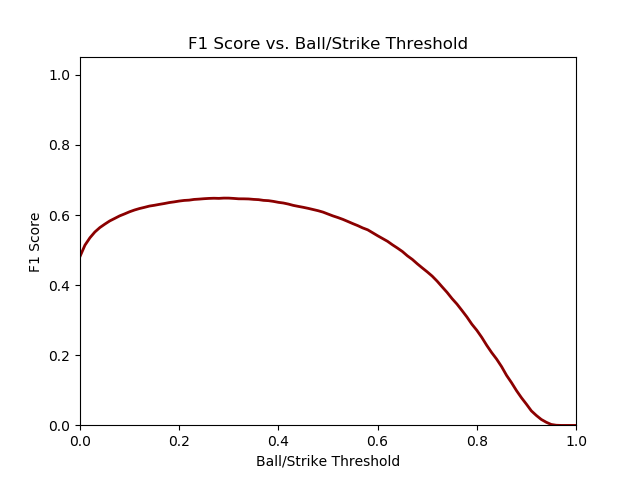
Recall that for each pitch, the output of the neural network is a value between 0.0 and 1.0, with values near 0.0 indicating the pitch is very likely a ball, and values near 1.0 indicating the pitch is very likely a strike. The above values were computed with the default ball/strike threshold at the middle value of 0.5, so if the neural network has an output less than 0.5, we called a ball, and if it has an output greater than 0.5, we called a strike. We have the ability to tune this threshold. Let’s try to maximize our F1 score. Here is a graph of F1 score vs. threshold:

Note that on this graph, a ball/strike threshold of 0.0 means we always call strikes, and a threshold of 1.0 means we always call balls.
It looks like we can improve our F1 score if we lower our ball/strike threshold (meaning to call more strikes than at the default setting of 0.5). Indeed, the maximum F1 score of 0.570 is attained at a threshold of 0.29. Here is the confusion matrix at that threshold:
| Deep Learning’s call (down) / Umpire’s call (right) | Strike | Ball |
|---|---|---|
| Strike | 11826 | 14239 |
| Ball | 3587 | 19166 |
The overall accuracy is 53.3 percent, the precision is 45.3 percent, and the recall is 76.7 percent. Whereas the previous system had a higher precision than recall, now things are flipped around, with this system calling more strikes than balls. Note that in improving our F1 score, our accuracy fell by quite a bit. However, this is not really a cause for alarm.
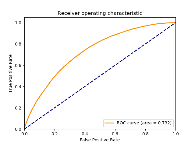
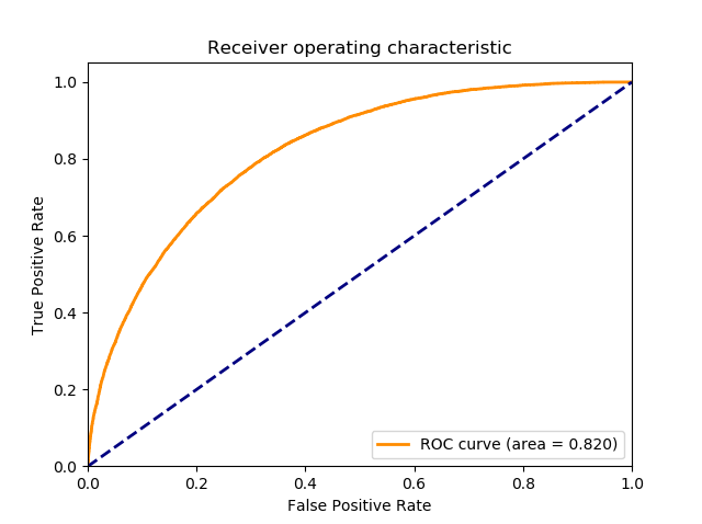
Looking at things at a slightly more general level, encompassing the whole range of thresholds between 0.0 and 1.0, here is the ROC curve (receiver operating characteristic curve), which yields an AUC of 0.732 (a perfect AUC is 1.0):
Incorporating optical flow images
At the end of my previous article, one proposal I had for improving the system was to incorporate optical flow images. I went ahead and did just that by utilizing the “Flownet 2” software package developed at the University of Freiburg in Germany. For each successive pair of frames in each 0.4-second truncated pitch video, I computed the optical flow image frame.
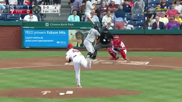
To get a sense of what these optical flow images look like, here is a full pitch video, with the corresponding optical flow video below it:
The color at each pixel indicates the direction of movement, and the intensity of the color at each pixel indicates the magnitude of movement. You can see the red streak that indicates the path of the ball, along with patches of color that indicate the movement of the pitcher, batter, bat, and catcher’s mitt. Below are a pair of frames with the ball in between the pitcher and the catcher; you can see the ball visible as a white spot in the original image and as a red spot in the optical flow image:

As it turns out, this optical flow software package was not able to detect the trajectory of the baseball in the majority of the videos. This is likely because the ball is a much smaller object compared to the players and umpires in the video, and the software was not trained to detect and track the movement of an object as small as a baseball. In videos where the ball was tracked, it yielded extra information that is be useful to the classification algorithm, and in videos where the ball was not tracked, the algorithm was really no worse off than it was before I introduced the optical flow images.
On the flip side, the trajectory of the catcher’s mitt was able to be detected in basically all of the videos. This information certainly is useful to the classification algorithm, both as a proxy for the ball’s location (in cases where the ball wasn’t tracked), and also to supply pitch-framing information. Furthermore, the movements of the bat, batter, and pitcher also were able to be detected in basically all of the videos, and supplying this information certainly can’t hurt. One interesting question that arises from this data is whether the extent of a batter’s checked swing influences the umpire’s decision to call a strike. (That is a question for another study.)
The optical flow image frames were put through the same Inception V3 CNN the original frames were put through. Afterwards, the 2048-element feature vector produced by the optical flow image frame was concatenated with the original 2048-element feature vector to form a new 4096-element feature vector. This process is known as “late fusion” (as opposed to “early fusion,” where the original image would be concatenated with the optical flow image and then the concatenated image would be put through the CNN). After these new feature vectors are computed, they are then sent as input into the LSTM RNN, just like in the original process.
With the optical flow image data added in, the new optimal F1 score is 0.649 (at a ball/strike threshold of 0.29) and the AUC is 0.820. Note that the fact that the same threshold of 0.29 was optimal was just a coincidence.
Clearly, we can see that the results are improved substantially by adding in the optical flow image data.
Expanding the data set
To finish this phase of the project, I decided to run my code and analysis on video data from the 2015, 2016, and 2018 regular seasons. I would expect that with more data, we have the potential to get better results.
Recall that in Part One of the project, I wrote that the slowest step in the data processing chain (by far) was using Openpose to compute the pose estimation of the pitcher’s body. I went back to that code and made several refinements and improvements to the algorithms. In addition, in the past few months since I originally started on the project, the authors of Openpose have improved things from their end. Combined, these changes allowed me to run the pose estimation step about ten times faster than before. This allowed me to run the pipeline on the other season’s video data much faster than before. (It still took a total of a couple weeks.)
With the processed data, I ran more experiments with the data from 2017 and 2018 combined (about 300,000 balls and 138,000 strikes), with data from 2016 to 2018 combined (about 462,000 balls and 214,000 strikes), and with data from 2015 to 2018 combined (about 625,000 balls and 288,000 strikes):
| Season(s) | F1 score | AUC |
|---|---|---|
| 2017 | 0.649 | 0.820 |
| 2017 and 2018 | 0.655 | 0.833 |
| 2016 to 2018 | 0.662 | 0.838 |
| 2015 to 2018 | 0.673 | 0.850 |
Between each consecutive pair of rows, you can see we have increased our success metrics by adding another year of data. However, it is clear this improvement is much smaller than the improvement we achieved by adding optical flow data. The marginal increase in fidelity is basically linear, but if you consider the order of magnitudes involved, by adding hundreds of thousands of data points we are only improving by a couple of percentage points. If we were to expand the data set further, I suspect we will hit the law of diminishing returns very quickly and get sub-linear marginal improvement in fidelity with each additional year of data. We almost certainly would have to add some new feature to our pipeline in order to get larger gains in fidelity.
Conclusion
In Part Two of this project, I showed several methods that improved our robot umpire system by quite a bit, and the results are better than what we achieved in Part One. As it stands right now, the fidelity of such a system still may not be quite good enough to be deployed in a live major league game, but with more work, I am confident we will get to that milestone in the future.
great work, but if went to this it would be the beginning of the end for mlb.
just like tennis eh?
Wut?
I sure hope this come to pass soon. It is really discouraging to study catcher defense and learn the most important contribution they can make is coercing an umpire into making the wrong call by “pitch framing”.
And some think stealing signs is unethical too.
We need this now. There are far too many bad umpires, and at least three who fully qualify as clowns. Just in the playoffs so far I have seen numerous badly missed calls, two of which I am convinced were intentional. It’s time to make baseball fair and honest for the first time: Robot umps now!! !
I’ve done some work on umpire strike zone replication, and at the risk of being a wet blanket, those AUC results are pretty poor compared to, say, just classifying based on historical ball/strike calls across MLB for each square inch in the front-of-plate z-plane using PITCHf/x data.
This is cool work and a nice example for training an ML model on video data, but in terms of actually building a viable robot umpire you’re really hamstringing yourself by not using a more appropriate dataset.
This is a fun project and thanks for the articles. I certainly learned plenty. But I don’t think it tells us a lot about the feasibility of robot umpires.
Your results are inflated by the fact that so many pitches are *clearly* balls or strikes; it’s accuracy on the pitches near the edge of the zone that is really the task here. How well would a system do that just took anything clearly more than a few inches within the zone and called it a strike, and everything more than a few inches outside the zone and called it a ball? That’s the baseline that AI, and umpires, should be compared to.
OTOH, *much* of your hard work was devoted to getting usable data out of lousy input. As you say, MLB can use camera capabilities and locations optimized for the task (plus lasers!), which you couldn’t. So the task is easier than what you’ve been wrestling with. Better data will beat more analysis every time.
To your comment, and Peter’s just before yours, I think the first real application of this won’t be for developing robot umpires, but for analyzing the drivers of good/bad catcher framing. If you can marry the video data analysis to PITCHf/x data, you will have additional data points that might describe why some ball and strike calls disagree with a PITCHf/x based formula for balls vs. strikes.
If this isn’t already being done by some MLB organization, I can see Roger getting a nice offer to join somebody’s analytics team to do this.
Absolutely! I think there are a lot of interesting applications for ML models applied to video data. I just think this one is pretty clearly sub-optimal… it simultaneously underutilizes the potential power of his video framework *and* does a poor job compared to existing methods.
Thank you all for your comments. I am not surprised that my system doesn’t work as well as a system based on PITCHf/x data. This project was more spurred by a “I wonder if deep learning could work on these pitch videos” attitude.