Finding Value in Fastball Mixing

Lance Lynn was among the best at mixing his fastball in 2014. (via Kathryn Prybyl)
Phil Hughes enjoyed a rather spectacular, albeit surprising, year with the Minnesota Twins in 2014. After averaging a 4.50 FIP over the three seasons prior, he posted a 2.65 FIP, a career low. Fueling this turn-around, among other things, was a more effective fastball — one that jumped in value from -13 runs to 15 runs (by pitch linear weights).
From 2011-2014, his fastball velocity has remained unchanged, hovering around 92 mph, and while his fastball percentage did take a jump in 2014—around 15 percent over the previous three-season average—that was surely not enough to justify a 30 run increase in its effectiveness. Presumably, if we don’t attribute this uptick in fastball effectiveness to random variation, Hughes must have changed his fastball usage drastically. As Eno Sarris noted, Hughes’ increased use of his cutter and curveball as primary offerings could explain his success and his uptick in fastball effectiveness overall. But was it the inclusion of the cutter and curveball that allowed Hughes to be more effective or was it the approach that those pitches encourage that made him and his fastball better?
Sure, it’s clear Hughes is due for some regression when you consider his fortunately low HR/FB percentage, but it’s not quite as clear whether his success can be considered a function of his change in approach. In fact, this is where the problem lies: Explaining pitch production, and, to a certain extent, how a pitcher uses his pitches in a given season isn’t easy given our normal assortment of statistics. In fact, when considering the fastball and its value, zone percentage (zone), fastball velocity (vFB), fastball percentage (FB%), and the like do little to describe how effective a pitcher’s fastball was that year.
In short, Hughes got me thinking about approach and our lack of available metrics that measure it. For instance, there is something to be said about the difference in approaches between a pitcher who throws five consecutive fastballs and follows that up with four change-ups and a curve, and a pitcher who alternates between fastball and change-up in a ten-pitch sequence. That would look like something like this (where “1” is fastball, and “0” is non-fastball).
Pitcher 1: 1111100000
Pitcher 2: 1010101010
Despite the clear differences in the way these two pitchers use and mix their fastballs, they both used the fastball 50 percent of the time. Say that the movement and velocity on their fastballs are similar. So these pitchers have similar fastball profiles, yet there is no evidence to suggest that they sequence, mix, and use the fastball in a similar way. Here, obviously, approach is much different than what the averages tell us on the surface.
It’s easy to fall into this way of thinking when we look at metrics that measure outcomes with respect to a specific pitch: whiffs per swing, batted ball per ball in play, zone percentage, and you name it. The problem here is that none of these really help to answer the question of why the fastball was effective, they only help to answer how it got outs. As you can imagine, it is hard to remove the process from the results when we view it only through this lens. That is not to say that there is no good way of measuring how a pitcher uses his fastball, besides anecdotal, or scouting information — which are both very good. But, since this is The Hardball Times, I would like to explore a way to quantify a pitcher’s approach. Today, my question is: Is there a way to measure how a pitcher was using his fastball, and mixing it, relative to his other pitches? I will show you that there is a relationship between fastball mixing and success.
Methodology
One way to measure approach is to look at observed randomness in a sequence. Identifying randomness of a binary bit sequence (a string of many 1s and 0s) is an activity with its fair share of applicable statistical tests. The National Institute of Standards and Technology (NIST) has recommended an assortment of statistical tests to assess the randomness of a binary sequence. In reality, these tests are meant to be applied to cryptography in order to assess the validity of a random number generator or to test the strength of a program’s security. So, it’s reasonable to be skeptical about the validity of these tests once applied to binary sequences in the scope of baseball. But we will do our best to make the application as smooth as possible.
In order to apply the NIST suite of tests we need to transform a pitcher’s pitch selection into binary elements. Using MLBAM pitch tags, we can code up all fastball pitch types as “1” and all other pitch types as “0”, then we can transform a pitcher’s pitch vector, FV, into a binary sequence:
FV= (Po, Po+1,…, Pn-1)
… where fastball pitch types are all fastball related pitch tags (Examples: FF, FT, FA, FS, FC, SI). All other pitches are deemed non-fastball—binning off-speed and breaking offerings together.
Now there are a few ways to make this work, so as to remove biases from this approach: we will isolate for pitchers who use one primary fastball to complement breaking and off-speed pitches. I chose an arbitrary 0.70 ratio of a pitcher’s primary fastball type to all other fastball types as the cut-off for our sample. This will remove pitchers who may use an alternate fastball that functions as a complementary pitch.
Now we could bin cutters with sliders, but while many cutters are similar to sliders in a pitcher’s arsenal, this assumption over an entire sample of pitchers may not be completely accurate. So instead, we will try to isolate for pitchers who are more or less binary in their approach—main fastballs and all else. The binary aspect of this approach is why I am putting it under the heading of “Pitch Mixing” and not “Pitch Sequencing.” This approach aims to find the optimal way to mix, or combine, disparate pitch types with the fastball, whereas pitch sequencing is the study of the optimal order in which a pitcher can throw his pitches.

Some disclaimers: This approach does not come without its fair share of assumptions and biases, even after correcting for a few. Of course, we can’t completely assume a pitcher’s mixing is a binary procedure—this is an overly simplified way to look at the optimal way to mix fastball and off-speed. We also have to be wary of the inaccuracy of pitch classification, which is far from perfect, for a pitcher over the course of a given season—especially if he is relatively new to the majors.
Most importantly, I have to note that pitch mixing is not completely independent; that is, the previous pitch has a slight effect on the probability of the next pitch. In other words, the probability of a fastball on pitch n given pitch n-1 is not equal to the expected probability of a fastball on any given pitch. But by applying the tests that we plan to use today, we are implicitly assuming pitches are independent—which may or may not be completely correct. So as to assume maximum independence, we will look at pitch mixing between similar counts.
If grouping by counts doesn’t make sense, think of it this way: we will look at the pitch vector of a pitcher for every count, C. Consider a vector of four consecutive “1s” in a three-ball, two-strike count. Each “1” or fastball in this vector would be more independent of each other than four consecutive ones in a sequential pitch vector (pitch 1, pitch 2, pitch 3, and so on), because there is less dependency on the previous pitch when we control for count. The advantage in looking at the mixing between counts is that it will allow us to apply the statistical tests to measure randomness and still meet all their conditions of independence. We can then take a weighted average of all counts to get a more accurate overall pitch mixing assessment.
At this point, it would be useful to know the point at which our binary pitch bit sequence stabilizes. That is, at how many pitches does the observed data from the pitch vector become more predictive of future classification than a league-average expectation? We can do this a variety of ways, but the most computationally basic way is to use split-half reliability between odd- and even-numbered pitches. There may or may not be bias in split-half analysis through even-numbered pitches and odd-numbered pitches, thus skewing the analysis; but for the sake of this article, it will be good enough to give us a rough estimate of a pitch cut-off point. For future implementation, a more accurate and much more complex method would utilize the Kuder-Richardson reliability formula—one that Russell Carleton has touted in the past.
Using data from 2014, I found how long it took for the binary pitch vector to stabilize for every pitcher of interest. Below is the graph of stabilization:
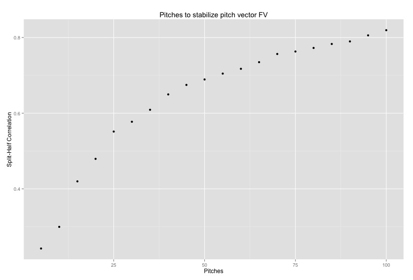
We are looking for the point where the split-half correlation exceeds 0.707 (0.707^2 is approximately an R-Squared of 0.50). As such, our pitch classification vector stabilizes fairly quickly, at around 55 pitches—the point where observed selection is just as reliable as league average selection in terms of future prediction.
Now that we discussed stabilization and independency of pitch classification, it’s time to move on to the statistical tests to measure randomness, or lack thereof, in a pitcher’s pitch mix vector. There are three tests that we will incorporate into our assessment: The Runs Test, The Cumulative Sums Test, and The Streak Gap Test.
Runs Test
The focus of the Runs Test is to test if the number of runs observed is unexpectedly above what would be expected in a random bit sequence. Here we define a run as a two consecutive like bits. For instance, consider the following bit sequence:
100101101
In our context, this is one fastball, followed by two breaking/off-speed pitches, and so on. Our Runs vector will look like this:
001000101
That means in our 10-pitch sequence we observed three runs of consecutive like pitches. Now, the next logical step is to test whether three runs out of 10 pitches could be observed in a random sequence. If that is unlikely, we expect a small test statistic. In simplest terms, NIST says this test is appropriate to detect if the “oscillation of zeroes and ones is too fast or too slow” for a random sequence. The larger the test statistic, the more evidence that it does not follow a random design.
Cumulative Sum Test
The Cumulative Sums test works in a similar way to the runs test, except that we look for the maximum cumulative sum of consecutive terms. To do this we transform the vector into “1s” and “-1s”, where “1” is a fastball and “-1” is a non-fastball. Next, we take the maximum cumulative sum of the transformed vector. Take for instance, the 10-pitch sequence of four fastballs followed by two non-fastballs, finished off with four fastballs:
1111001111
Then we transform this 10-pitch sequence:
1111-1-11111
Lastly we take the sum of consecutive terms:
S1=1=1
S2=1+1=2
S3=1+1+1=3
S4=1+1+1+1=4
S5=1+1+1+1-1=3
S6=1+1+1+1-1-1=2
S7=1+1+1+1-1-1+1=4
S8=1+1+1+1-1-1+1+1=5
S9=1+1+1+1-1-1+1+1+1=6
S10=1+1+1+1-1-1+1+1+1+1=7
The maximum of the cumulative sum, from partial sum 10 (“S10”), is seven. The test statistic is the absolute value of the maximum cumulative sum divided by the square root of length of the pitch vector. The test-statistic gives us an idea if the maximum cumulative sum is unlikely to occur given that the sequence is random.
Streak Gap Test
This last method is not suggested by NIST. Instead, I have adapted an approach to assess the streakiness of a player’s hitting outcomes used by Max Marchi and Jim Albert in Analyzing Baseball with R. The idea is to take the squared sum of the gaps in between 1s and 0s in a vector and identify if the squared sums (S) is larger than one would expect if every possible combination of 1s and 0s was equally likely. As such, we take any vector and simulate the test statistic 1,000 times from a sampled vector of equal length. We then compare the distribution of S given a random simulation versus the observed S in the actual vector. Take for instance the following 10-pitch sequence:
100101101
S for the following vector is 6 (2^2+1^2+1^2). We then would randomize this vector one thousand times, and compare the observed S statistic to the expected S statistic. The test statistic is the Z-score of the S-stat given the mean and standard deviation from the distribution of the simulated S-stat.
Results
Year-to-Year Correlations of Metrics, Predictive Value, Summary Statistics
Below is a table with the summary statistics for each metric—Runs, Streaks, Cumulative Sums (CSUM) — for all pitchers since 2011 with at least 55 pitches in the given season:
| Summary Statistics, 2011-Present |
|---|
| Metric | Mean | STDEV |
| CSUM | 5.66 | 3.80 |
| Runs | 10.61 | 50.03 |
| Streaks | 0.56 | 1.69 |
And a Correlation Matrix between the metrics:
| Correlation Matrix, 2011-Present |
|---|
| Metric | CSUM | Runs | Streaks |
| CSUM | 1 | 0.38 | 0.14 |
| Runs | 0.38 | 1 | 0.02 |
| Streaks | 0.14 | 0.02 | 1 |
CSUM and Runs have the closest relationship — which makes sense because they both measure consecutive bits in a string. Meanwhile, Streaks and Runs have almost zero relationship, whereas CSUM has comparatively larger relationship with Streaks.
CSUM is by far and away the most descriptive of the three metrics:
| CSUM, 2011-Present |
|---|
| CSUM | wFB | FIP | vFB | FB% | Pitch Value (not Fastball) | Count |
| Z >= 2 | 6.39 | 3.39 | 91.97 | 0.57 | 7.78 | 67 |
| Z <= 2 | -0.65 | 4.32 | 91.76 | 0.54 | 0.07 | 1,435 |
In the distribution of the z-score of CSUM, while it is skewed left, those who find themselves in the right tail tend to be far and away more productive with their fastball and, overall, almost a run better in FIP. CSUM has a 0.28 correlation with wFB/C, and a -0.30 correlation with FIP on the entire sample (all pitchers since 2011 with at least 55 pitches in a given season). In this sample, CSUM is more productive at describing wFB/C, wFB, and FIP than zone percentage, fastball velocity, and fastball percent. So while, the relationship is not strong in general, it can be seen as relatively strong.
It’s important to note that CSUM has a strong relationship with the number of pitches in a string but has a relatively small relationship with fastball percentage overall. And in a multiple regression of wFB, CSUM, std_csum, fastball velocity, and fastball percentage, we can explain 19 percent of the variation in next year’s weighted fastball. So, it can be a useful tool when used to supplement the measures we already have.
From here on we will use CSUM as our primary mixing metric, and our fastball approach proxy.
Number of Disparate Pitch Types, Secondary Fastballs, and Their Effect on Pitch Mixing
We want to test if the number of pitches a pitcher uses, or incorporates, in a given season can influence our mixing metric. And, as shown below, CSUM is only slightly explained by the regression:
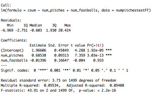
An R-squared of five percent means that only five percent of the variation in CSUM is measured by the number of pitch types and number of fastball types used by any given pitcher. Of the two variables, number of pitches was a significant variable in explaining CSUM, where as number of fastballs was nowhere close.
Team Switchers and Approach
When evaluating the usefulness of any metric I always like to look at the effect changing scenery has on the year-to-year correlation. If we see that those who changed scenery saw a large difference in their year two mixing, we can begin to deduce that there is some confounding variable affecting the year-to-year correlation of the CSUM — whether it be the catcher, the team-ideology, or something else. In this case, likely something outside the pitcher’s immediate control severely affects the way he mixes his fastball. If there is little change, and CSUM remains skill-based even for those who switched teams, then we can assume pitchers have some control over their mixing.
From 2011-2014, 125 pitchers switched teams during the sample. The first R-output summary shows the results of the linear regression for team-switchers:

Here the R-squared of the regression was around 43 percent. That means 43 percent of the variation observed in year-two team switchers’ approach was explained by year-one’s mix metric.
And this output shows the year-to-year correlation of CSUM for non-team-swichers:
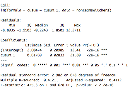
As shown above, there was no real change in the strength of the relationship (43 percent versus 41 percent). Surprisingly, team-switchers had slightly more control compared to those who remained with the same team. This affirms that this may be a pitcher-specific skill that is not necessarily affected by organizational ideology changes or the like. Obviously, this is an oversimplified look at the effect on team factors on a pitcher’s mixing and fastball usage, but it gives us a good idea that the effect is not big enough to affect our analysis.
Pitchers who mixed the most in 2014
By weighted accumulative CSUM, weighted average of CSUM in each count, below are the streakiest pitchers with their pitch mixing.
| Streakiest Pitch Mixers, 2014 |
|---|
| Rank | Name | CSUM | wFB | FIP |
| 1 | Phil Hughes | 21.58 | 15.27 | 2.65 |
| 2 | Clayton Kershaw | 19.89 | 19.18 | 1.81 |
| 3 | R.A. Dickey | 19.71 | -1.30 | 4.32 |
| 4 | Charlie Morton | 16.63 | 2.22 | 3.72 |
| 5 | Shelby Miller | 16.56 | 13.35 | 4.54 |
| 6 | Lance Lynn | 15.81 | 10.42 | 3.35 |
| 7 | Kenley Jansen | 15.53 | 8.13 | 1.91 |
| 8 | Chris Young | 15.15 | -8.40 | 5.02 |
| 9 | Zach Britton | 14.68 | 18.36 | 3.13 |
| 10 | Danny Farquhar | 14.61 | 2.22 | 2.86 |
| 11 | Kelvin Herrera | 14.55 | 11.40 | 2.69 |
| 12 | Burke Badenhop | 14.36 | 6.87 | 3.08 |
| 13 | Danny Salazar | 14.10 | -3.11 | 3.52 |
| 14 | Danny Duffy | 13.95 | 13.57 | 3.83 |
| 15 | Brandon League | 13.83 | -1.00 | 3.40 |
| 16 | Jordan Zimmermann | 13.63 | 14.62 | 2.68 |
| 17 | Jared Hughes | 13.45 | 4.19 | 3.99 |
| 18 | J.A. Happ | 12.86 | 2.12 | 4.27 |
| 19 | James Paxton | 12.27 | 9.83 | 3.28 |
| 20 | Cole Hamels | 12.25 | -0.26 | 3.07 |
| 21 | Ronald Belisario | 12.10 | 1.82 | 3.54 |
| 22 | Tommy Kahnle | 12.00 | 4.49 | 4.02 |
| 23 | Trevor Rosenthal | 11.97 | 1.75 | 2.99 |
| 24 | Gerrit Cole | 11.93 | 4.59 | 3.23 |
| 25 | Brian Schlitter | 11.88 | 0.53 | 3.61 |
As alluded to earlier, Hughes saw a huge change in CSUM from 2013 to 2014, when he led the league in fastball “streakiness.” Of note: to interpret these numbers, the larger the CSUM, the less likely this pitcher’s fastball vector is observable in a random sequence of equal length. Of course, all these pitchers are in the right tail of the distribution and they are of reasonably higher quality than the rest of the sample when it comes to fastball quality and FIP-based performance.
Pitchers who mixed the least in 2014
Now, let’s go the other way.
| Least Streaky Pitch Mixers, 2014 |
|---|
| Rank | Name | CSUM | wFB | FIP |
| 1 | Troy Patton | 0.39 | -0.82 | 4.20 |
| 2 | Ryan Dennick | 0.40 | -1.64 | 9.99 |
| 3 | Tyler Clippard | 0.42 | 5.79 | 2.75 |
| 4 | Drew Rucinski | 0.51 | -1.06 | 2.18 |
| 5 | Chris Heston | 0.61 | 0.88 | 3.32 |
| 6 | Joba Chamberlain | 0.63 | -1.38 | 3.16 |
| 7 | Daniel Coulombe | 0.64 | -2.07 | 5.67 |
| 8 | Collin McHugh | 0.76 | -5.60 | 3.11 |
| 9 | Rich Hill | 0.77 | -1.04 | 3.69 |
| 10 | C.J. Riefenhauser | 0.82 | 0.29 | 4.07 |
| 11 | Josh Outman | 0.83 | 0.81 | 4.83 |
| 12 | Lucas Luetge | 0.85 | -1.09 | 7.58 |
| 13 | Yusmeiro Petit | 0.85 | -3.86 | 2.78 |
| 14 | Bruce Chen | 0.87 | -3.03 | 4.58 |
| 15 | Shawn Kelley | 0.88 | 0.47 | 3.02 |
| 16 | Jeff Francis | 0.89 | 1.76 | 4.18 |
| 17 | John Lannan | 0.94 | -4.05 | 13.38 |
| 18 | Sean O’Sullivan | 0.94 | -2.40 | 5.58 |
| 19 | Al Alburquerque | 0.99 | 0.22 | 3.78 |
| 20 | Hunter Strickland | 1.00 | 1.16 | 0.56 |
| 21 | Chris Leroux | 1.03 | -0.71 | 3.13 |
| 22 | Ryan Rowland-Smith | 1.06 | -1.28 | 2.31 |
| 23 | Felipe Paulino | 1.08 | -5.82 | 7.99 |
| 24 | Rudy Owens | 1.11 | -2.69 | 6.66 |
| 25 | Luke Putkonen | 1.18 | -3.31 | 15.51 |
As seen above, the overall quality of fastball and FIP-based performance is less for those who mixed more randomly (or less “streaky”). Most everyone on this list is a reliever, with a quality starter (Colin McHugh) and a spot-start/relief-king (Yusmeiro Petit) sprinkled in between.
Conclusions
At the very least, CSUM gives us a reasonable metric that can tell us something more about how a pitcher actually used his fastball—a metric that is at once descriptive of approach and production (in terms of describing wFB and FIP). Whether the benefits of having a higher CSUM, and being less random with fastball mixing, is independent of other factors is something I hope to address in future research.
In short, what does it tell us?
- There is approximately zero relationship between fastball percentage and the mixing metric (CSUM)
- CSUM is more descriptive of fastball production and FIP than fastball velocity, fastball percentage and zone percentage
- CSUM has a year-to-year correlation of 0.64 (r), strongly skill-based
- Fastball pitch mixing is not as affected by number of disparate pitch types (fastball and non-fastball) as previously suggested; perhaps, it is more of a function of the quality and confidence of those separate pitches.
- Team-switching did not have large or noticeable affect on a pitcher’s measured fastball approach; in fact, team-switchers had a stronger year-to-year relationship
In the future, using an improved CSUM, or something very similar we can look into:
- The effect of catchers on pitchers’ pitch mixing
- Candidates for decline or breakout when considering a change in stuff that is not met with subsequent changes in approach to accommodate/adjust
- The times-through-the-order effect on pitch mixing
Next Steps
- Improve weighting system between counts: Should pitcher counts be weighted more to improve usefulness of the metric?
- Use Block Test to remove pitchers who have string-of-pitch-classification issues from sample
- Control for base-state-out, batter quality
References and Resources
- Eno Sarris, FanGraphs, “Phil Hughes Finally Found the Right Breaking Balls”
- National Institute of Standards and Technology (NIST), “Guide to the Statistical Tests”
- FanGraphs, “Pitch Type Abbreviations & Classifications”
- Russell Carleton, Baseball Prospectus, Baseball Therapy: It’s A Small Sample Size After All
- Max Marchi & Jim Albert, Analyzing Baseball Data with R
- Charmaine Kenny, Random.org/Trinity College Dublin, “Random Number Generators: An Evaluation and Comparison of Random.org and Some Commonly Used Generators”
- Random.org, Statistical Analysis
- Louise Foley, Random.org/Trinity College Dublin, Analysis of an On-line Random Number Generator
- *ALL R CODE IS LOCATED HERE*
- *ALL DATA IS LOCATED HERE*
Max – has Vince Gennaro snapped you up yet as an instructor for his Diamond Dollar competition?
http://www.hardballtimes.com/digging-for-diamonds/
TZ — as of right now, nope.
Very interesting work.
What I wonder about though – is at both extremes, predictability is higher than in the middle. In other words, pitchers which streak and pitchers which deliberately don’t streak are equally predictable in a certain, though different sense.
While the methodology used is understandable, it is a pity because pitchers who are infamous for certain pitches like Sergio Romo with his no dot slider are excluded.
I think there is some good stuff here, but I am a little lost (suggestion to Max: DUMB down your articles – this is NOT a scholarly journal!).
A high CSUM number means MORE or LESS randomness? “Streaky” implies less randomness, right? So the first table of the “streakiest” pitchers have the BEST fastballs? But they are predictable, right? Why would they have the best fastballs?
Do these methods take into consideration the overall frequency of fastballs thrown? For example, if pitcher A throws 50% FB, a typical run/vector might look like this:
1000110100011
If pitcher B throws 90% FB, a typical vector might look like this:
11111111111101
What would CSUM say about these two pitchers?
MGL,
Thanks for reading through the density— I’m definitely working on dumbing down my articles 🙂
So a high CSUM would mean *less* randomness, so “streaky” means they string their fastball together more than one would expect in a random mix approach. (That is not to say the difference is statistically significant, that is another conversation).
For your first pitch vector the CSUM is around 0.8… The second has a CSUM around 2.5.
I would say that may point to a bias for high fastball usage pitchers; but, the funny thing is that FB% had little to no correlation with CSUM. That being said, the length of the vector explained a sizable portion of CSUM (but that might have to do with the idea that length of the pitch vector is in the denominator of CSUM). That may be a problem in term of selection bias.
The one test not used (Block Test, see references if interested) does adjust better for overall frequency, so I’d like to incorporate that in the future. My next step is to explicitly measure “uncertainty”—perhaps similar to Rob Arthur’s Entropy method (http://www.baseballprospectus.com/article.php?articleid=22758)— and see the relationship between this measure of randomness and “ability to guess correctly”.
My interpretation for why these pitcher’s fastballs are better is 1) better quality of other pitches (see table), for whatever reason, that seemed to be a trend in streaky pitchers; 2) higher level of confidence and quality in terms of fastball… And I will have to reserve further judgement until I find a way to adjust for catcher influence—something that I suspect matters, like in most battery outcomes—and look at specific pitch combinations that may promote a higher level of streakiness. Someone pointed out that the less streaky pitchers mostly were fastball-change guys, etc.
It’s obviously open to interpretation, at this point, but I hope this is an area we focus on exploring more.
Great work.
Two questions. 1) Isn`t is correct that the CSUM is calculated around the pitchers` average FB%, not just 50%. 2) What is exactly mean by “weighted average of CSUM in each count”. Can you show me some examples?
Thanks…
Weighted average:
My CSUM in count 2-0 (C1) is 2.5.
My CSUM in count 2-1 (C2) is 1.0.
If these are the only two counts I threw in then CSUM = ((pitches in C1*CSUM in count 1)+(pitches in C2*CSUM in count 2))/(pitches in count1+pitches in count2))
I should mention that this weighted average is assuming all counts are equal, for the sake of simplicity—which is ironic.
Anyways, I am experimenting with the weights so that the CSUM (or any mixing metric) is optimally descriptive of run prevention and fastball production.
This has some interesting ideas about pitch mixing and testing randomness, but I don’t think the Cumulative Sum test is necessarily the proper tool for that in this case.
The cumulative sum test described on the NIST site is really only designed to test randomness assuming p=.5. It doesn’t work for testing if a sequence of of 1s and 0s appears random given different probabilities for 1 and 0 (i.e. if a pitcher’s fastball percentage isn’t near 50%, his sequences will probably fail the cumulative sum test for randomness, given you observe enough pitches).
This happens because the test is based on the assumption that the cumulative sum for random data should stay within a certain range of zero most of the time, which is only true if p=.5. If p=.6, for example, then you would expect the cumulative sum to keep growing the more observations you get even if the data is random (since there will be about one-and-a-half 1s for ever -1 in the series). The test statistic will just keep getting higher and higher the more data you observe.
The NIST site gives an example illustrating this (which is kind of hard to follow since it’s documentation for software and not really a teaching example).
The example runs the test on four sets of randomly generated data, using p=.5, p=.58, p=.65, and p=.85 to each generate 200 random observations. Even though all four sets of data were randomly generated by the same function, the data fails the test worse and worse the further p gets from .5. The test-statistic goes from ~0.8 for the data generated from p=.5 to ~2.2, 4.3, and 10.8 for p=.58, .65, and .85 respectively.
As a result, a high test statistic in the cumulative sums test can be indicative of either:
1) data that is not distributed randomly
2) data where p differs significantly from .5, whether it is random or not
3) data where p differs at all from .5 and has a lot of observations, whether it is random or not
And the further you get from p=.5, or the more observations you get (unless p is actually .5), the larger the test statistic will end up.
Unfortunately, that means this test is not actually useful for measuring randomness in pitch vectors, because the last two factors are going to dominate the results. This is why you see a strong relationship between CSUM and the number of pitches in the series (theoretically there should also be some relationship between CSUM and FB% as well, but from your results it sounds like that effect is being swamped by the effect of the varying number of pitches thrown by pitchers in the samples).
This is also why the leaderboard shows a lot more starters with high IP totals (or relievers with extreme FB%, like Kenley Jansen) with the highest CSUM. It’s also why a lot of the pitchers with the lowest CSUM are relievers with low IP totals or pitchers with a FB% near 50%, like Yusmeiro Petit.
It’s also likely that the relationship between pitches thrown and CSUM is a major factor in CSUM standing out from the other randomness tests you looked at: it’s not that CSUM is telling you more about pitch mixing, but that the test statistic is picking up a lot of other information (probably mostly from the number of pitches thrown by each pitcher in the sample) that the other randomness tests aren’t.
I do think running randomness tests on sequences is a really interesting idea, and a good starting point for trying to find effects of pitch mixing or sequencing. Unfortunately, any effects found are probably going to be a lot more subtle than this.
Thanks Kincaid, great comment…
Possible ways to address the p > or < 0.5 problem: 1) Take CSUM and simulate test statistic X number of times given a vector that is randomized so that all combinations are equally possible for that length and P(1)—similarly to the Streaks test. This way we standardize CSUM with an expected CSUM for that p. 2) Find better way to measure randomness , using test that better adjusts for variations in p and (1-p), and where vector length has little relationship to test statistic. I do think that the problems you brought up are valid and something that needs to be address moving forward. That being said, I do think that ideologically it makes sense to have a bias towards high fastball usage pitchers...maybe not to this extent, but to a certain extent.. I plan to move forward with this, your comment was definitely informative in which direction that will be.