Going Deep on Goin’ Deep

The impact of Denver on launch angle and distance is apparent. (via bp6316)
Over the years I have been studying the physics of baseball, I have been totally fascinated with baseball aerodynamics. In a simple Physics 101 world, where the effects of the atmosphere are neglected, baseball trajectories are pretty boring. But we don’t live in such a simple world, and the atmospheric effects of drag and lift play a crucial role in the flight of a baseball.
When PITCHf/x data first became public in 2007, that system produced a veritable bonanza of information that has helped considerably with our quantitative understanding of the effects of drag and lift on a pitched baseball. But after a while those kinds of trajectories get pretty boring too, since they mostly follow a straight line, with just a little bit of deviation due to the combined effects of gravity and spin.
Far more varied, and therefore more interesting, are the trajectories of batted baseballs, which run the gamut from line drives (which are sort of like pitches) to fly balls to pop-ups. If the goal is to understand the atmospheric effects with quantitative precision, it is necessary to investigate all these varied kinds of trajectories. With the advent of Statcast, we now have the opportunity to do just that.
In this article, I will use Statcast data to take a first look at batted-ball trajectories, with the goal of developing an aerodynamics model, including the effects of drag and lift, based on the variation of flyball distances as a function of exit speed, launch angle, and air density. The data used in this study consisted of exit speeds, launch angles, and distances of approximately 80,000 batted balls from the 2015 season.
Although the spray angle was also part of the data set, it was not used in the analysis I present here. Since the home-field and game time temperature for each batted ball were also known, it was straightforward to calculate the air density, assuming standard atmospheric pressure and 50 percent relative humidity, neither of which I had access to.
Let me start with the overview shown in Figure 1.
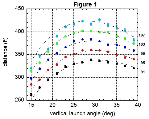
For this analysis, I considered only flyball hits for which the air density was close to the major league average. In particular, extreme elevations (e.g. Denver) and temperatures were excluded. In effect, I am trying to get an overview without the added complication of extreme atmospheric conditions. The plot shows average flyball distances and their standard error as a function of launch angle for various values of the exit velocity.
These data show quantitatively what we probably already knew, at least qualitatively. Namely, flyball distance reaches a maximum at launch angles in the vicinity of 25-30 degrees, with the angle decreasing slightly as the exit speed increases. Moreover, distances increase with exit speed at the rate of about five feet for each one mph increase in exit speed.
I have done this kind of analysis previously using HITf/x data, combined with independently measured home run distances, and found that an exit speed/launch angle of 100 mph/26 degrees leads to a mean distance of 405 feet, over 20 feet greater than found in the present analysis. The problem is a well-known issue with HITf/x exit speeds, which are measured at a distance somewhat removed from the ball-bat impact point, resulting in their being systematically underestimated. A 20-foot discrepancy corresponds to an underestimation of exit speed by about four mph.
These data are extremely valuable in developing and fine-tuning an aerodynamics model for the flight of the baseball. The important components of such a model are drag (i.e., air resistance) and lift (which results from the backspin). I use a model with five parameters that can be adjusted to best fit the data shown in the plot. Three of these parameters relate to drag and how it depends on the speed and spin of the baseball. The other two are used to specify the rate of backspin as a function of exit speed and launch angle.
The resulting model is shown by the dashed curves, which faithfully reproduce many of the features of the data. In particular, the model accounts for the slight shift in the peak of the distributions to smaller launch angle as the exit speed increases, a consequence of the increase of drag with speed. A notable exception to the good agreement is at the highest exit speed and angles below about 22 degrees, where the data fall distinctly below the curve and even appear to be discontinuous. Given that most things in nature behave smoothly, the data look suspect to me, but any stronger conclusion will have to await more data.
Figures 2 and 3 show mean distances for fly balls hit with an exit speed in the range 101-105 mph and with launch angle in the range 25-30 degrees.
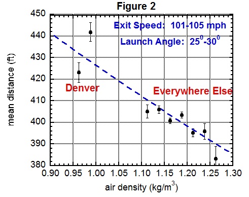
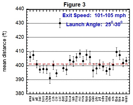
Figure 2 plots the mean distance versus air density along with a dashed line showing the model calculation. Interestingly, in Figure 2, both of those points on the left are Denver, as there is variability in the air density due to temperature. Figure 3 plots the mean distance for each major league stadium, with Denver the clear winner at 430 feet, compared with 401 feet for the average of the other stadiums, indicated by the red dashed line. The Denver effect is huge!
Since the model is an excellent representation of the data, we can use it to draw some interesting conclusions about how flyball distance depends on the various atmospheric effects. Some of these effects are shown in the table below, all calculated relative to 401 ft, which is the major league average distance (Denver excluded) for exit speed 101-105 mph and launch angle 25-30 degrees.

I next want to examine the Denver effect in more detail. To that end, Figures 4 and 5 compare distances in Denver with those at sea level, where the latter actually refer to air densities in the range 1.15-1.20 per cubic meter (or, kg/m3).
| Atmospheric Effect | Change in Distance |
| 10-degree increase in temperature | 3.3 ft |
| 1000 ft increase in elevation | 5.9 ft |
| 50% increase in relative humidity at 750 ft | 0.9 ft |
| 5.0 mph out-blowing wind | 18.8 ft |
Figure 4 shows distance versus exit speed for launch angles in the 25-30 degree range, while Figure 5 shows distance versus launch angle for exit speeds in the range 101-105 mph. As before, the lines are the model calculation.
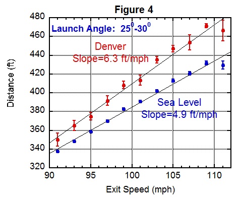
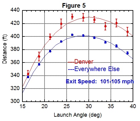
From Figure 4 we learn that the slope of distance versus exit speed is larger for Denver than at sea level, so that the Denver effect increases from about 19 feet at 91 mph to about 32 feet at 110 mph. From Figure 5 we learn that the distance peaks at a bit larger launch angle in Denver than it does at sea level. These results make sense physically, as reducing the air density at higher elevations pushes the trajectories closer to those expected in a vacuum, where distances increases much more rapidly with exit speed and peak at 45 degrees. The aerodynamics calculation nicely accounts for both of these features.
Another interesting comparison is Arizona and San Francisco, shown in Figure 6.
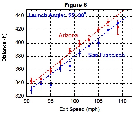
Arizona is about 1,000 feet higher in elevation than San Francisco and has an average temperature about 17 degrees warmer, both of which contribute to a lower air density and therefore a longer distance, just as shown in the plot. Once again, the calculation agrees with the general trend of the data.
But not everything is as well understood. As an example, consider Figure 7, which compares Tropicana Field with Wrigley Field.
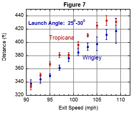
These two venues have mean air densities that are nearly identical, yet the data show the ball carrying measurably better at the Trop, by an average of over 10 feet. Perhaps we are seeing the net effect of an in-blowing wind at Wrigley, noting that no wind is expected at the covered Trop.
Finally, I want to take advantage of the fact that we have an aerodynamic model that accounts for most of the features of the data to investigate how flyball distance depends on the amount of backspin, here for a fixed exit speed of 103 mph and launch angle of 27 degrees. The results are given in the table below. They show that distance increases rapidly as the backspin increases from zero but eventually saturates, with very little gain in distance for spin rates exceeding about 1,500 rpm. The reason for the saturation is partly because air drag increases with increasing spin, essentially canceling the increase in lift.
| Backspin Rate (RPM) | Distance (FT) |
| 0 | 336 |
| 500 | 368 |
| 1,000 | 386 |
| 1,500 | 395 |
| 2,000 | 400 |
| 2,500 | 403 |
| 3,000 | 403 |
Before concluding, it is useful to remind the reader that the analysis considers only average distances for given values of exit speed and launch angle and that actual distance may vary. One reason for variation might be wind. Another might be variation in the drag properties of individual baseballs, which is a topic I addressed in a previous article and which can lead to a significant variation in distance.
I very much look forward to continuing my analysis to fine-tune the aerodynamics model. The work presented here was “two-dimensional,” in that the spray angle was ignored. Including the spray angle, both at impact and at the landing point, allows for the determination of the rate of side spin on the batted ball. Moreover, using the spin measured directly from the Trackman device — an integral part of Statcast — as well as the hang time, should allow better determination of the lift properties of the trajectory. There is still lots to do and, hopefully, lots of data to help do it.
Do the exit velocities themselves vary by ballpark, all other factors being equal? I remember seeing slightly higher exit velocities at Coors from the publicly available data on Baseball Savant from the 2015 season, but wasn’t sure if this was related to the limitations of that data set.
Great stuff as usual!
Fascinating read, as usual. Have a couple questions regarding “Figure 3”.
1) Do spin rates have an effect on this? I.e. do pitching staffs in those ballparks have backspin-suppressing abilities?
2) Is it likely that a lot of the variation could just be quirks with the methodology that will get fixed over time? I.e. I assume it calculates based on distances from each camera, which are not uniform ballpark to ballpark and even small variations in the distance estimates can produce consistently biased results.
tz: If you compare distribution of exit speeds for Coors vs. everywhere else, there are small differences, with the Coors mean value=88.8 and everywhere else mean value=88.4. If you examine the mean exit speed for every ballpark, you find quite a scatter, from a low of 87.0 in Cincinnati to a high of 90.2 in Arizona. I have no simple model to explain those differences.
Eli: (1) I doubt spin rates explain much of the variation in Figure 3, based on the information about how spin affects distance in the 2nd table. Aside from that point, your question about pitchers abilities to suppress backspin is an interesting one, although I have no quick answer. I would expect pitch location would have an effect, since it is hard to “get under” a ball that is already low. But it would make for an interesting study to examine how different pitchers/pitches affect the spin of a batted ball.
(2) I think a lot of park-to-park variation can be accounted for simply by air density, primarily due to elevation but partly due to temperature. My confidence in that comes primarily from the regularity shown in Figure 2. The Statcast system uses both the Trackman radar and cameras. For home runs, I am pretty sure that it is the radar that determines the distance. For other balls in play, I don’t know which is used. Ideally, both would be used, with one as a cross check on the other.
Alan – Interesting article as usual from you. There are weather archives available on the net that give temperature, humidity ,barometric pressure, wind speed and direction on an hourly time period for most if not all major league cities. There are sometimes more than one weather collection site so even though some conditions may not be exactly the same as in the ballpark they should be closer than the data data provided by Retrosheet for things like temperature, humidity and barometric pressure. Wrigley field is famous for its different playing conditions when the wind is blowing in as opposed to when the wind is blowing out so its not a surprise to see distances lower there on average.
Did the data you used from StatCast indicate which fly ball landing distances were tracked the entire flight of the ball and which were unable to track the entire flight and used an estimated landing location? Since they were using the Trackman system I am assuming that they still need to do this for some of the higher angle fly balls just as you found during your Houston research.
Indeed, the NOAA hourly data can give you pretty good inputs for temperature and pressure, as long as you use the right station. Many cities have more than one reporting station, and port cities in particular can have several that vary considerably. Seattle for example has one at SeaTac, which is nowhere near Safeco, and another downtown on top of a skyscraper which is only vaguely correlated with the conditions felt on the field; fortunately there’s also a waterfront “ferry terminal” station that is just a few blocks from the ballfield. (Safeco itself has its own weather station, complete with anemometer and barometer, but as far as I know the data it gathers is proprietary; I’m not sure if the team even uses it, or if it’s strictly for the benefit of the roof operator.)
Alan – http://www.ncdc.noaa.gov/qclcd/QCLCD this is a link to monthly data from Denver for August 2006. They also provide the same data in comma separated value format for easy loading into spreadsheets.
Peter: Thanks. The most important missing ingredient in analysis is the air pressure, and that really ought to be included. I will have a summer research student that I will put on that project. On the other hand, wind is very difficult to take into account, since the speed and direction can be different at different locations and heights in the ballpark.
I did not have access to the “last tracked distance” data from Statcast/Trackman. I simply took the distances at face value, hoping that they are correct on average. As we know, Statcast in 2015 sometimes disagreed with ESPN Home Run Tracker on home runs, sometimes by a significant amount. The significant ones are almost always attributed to incomplete tracking, for which the extrapolation algorithm that was used was not working well. Hopefully that has been fixed for the upcoming season.
Well if the media gets ahold of this, the Rockies will never have another MVP. I mean Arenado hit .287 with 42 HR (22 on the road mind you) and 130 RBI and I don’t believe he barely cracked the top 10. Yes Harper definitely deserved it, not saying that. Too bad notgraphs isn’t around anymore otherwise one could calculate what it would take for a Rockies player to win MVP lol
Alan,
Great stuff as always! (Anyone who needs a lesson on how to write in such a way that you clearly explain complicated stuff to a layperson needs to read Alan.)
I sent you an email regarding the NOAA data (air pressure, etc.).
I was also surprised at the Tampa data. Since it is an indoor stadium 100% of the time, how does that affect the air pressure/density? I understand that it is tricky to infer the air pressure inside of a building, especially when it is heated or air conditioned (forcing air into the building changes the pressure?).
We would expect the distance at Tamp to be low since it is at sea level and the temp is around 72 all the time I think.
And why did you only compare it to Wrigley Field which definitely has a problem with wind (BTW, if anything, the average wind at Wrigley is blowing out). Why not compare it with other parks with similar temp and altitude?
Also, you have a 19 foot affect for 5 mph wind? That seems like a lot. 5 mph is barely blowing at all. Is the affect linear or roughly linear? If yes, that implies that a 25 mph wind means almost 100 feet in distance which can’t be right.
MGL:
Looking at this first chart, and we see that 4 mph of launch speed adds around 20 feet in distance.
I presume therefore that if you have a 5mph wind that it has a somewhat similar effect. That is, a launch of 90mph with 5mph wind, or a launch of 95mph with no wind is somewhat similar? Is that what Alan is suggesting?
That would suggest a constant wind flow. Since Alan’s numbers are saying 5mph for 18 feet for wind (compared to 4mph for around 20 feet for human swing), there must be some non-constant wind flow?
Just guessing out loud here…
Tom, things are more complicated than you are describing. The way wind enters into a trajectory calculation is through the drag and lift, both of which are proportional to the square of the speed of the ball with respect to the air. That’s a mouthful. So, the initial drag on a 100 mph ball with no wind is identical to the drag on a 95 mph ball with a 5 mph following wind. In both cases, the velocity of the ball with respect to the air is 100 mph. But the equivalence of the two situations changes as the ball loses speed (both due to drag and due to gravity). Net result is that the 100 mph/no-wind ball travels farther than the 95mph/5mph wind ball.
When I want to figure out these things, I resort to my Trajectory Calculator (or something similar). There is no simple way that I know of to get the answer otherwise.
Alan, excellent, thanks. Based on your numbers you’ve published, while not 1 to 1, it seems about 3-4 mph of exit velocity is equal to 5mph of wind. Granted there’s more variables to it, but just to answer MGL’s surprise at the numbers, I think it gives us a ballpark number to appreciate how much impact the wind can have, even if it’s a light breeze.
I think it’s easier to see/believe with golf, where a decent wind is going to add 10-20% of distance to your drive. And maybe it’s easier to believe there because the ball is so tiny, and it seems that it should “carry” on the wind with much less resistance.
Interesting how real-life experiences can inform or distort our expectations. I’m not a golfer, but I would anticipate the opposite — that a golf ball would more easily “punch through” the wind than a baseball. My reasoning: golf balls are denser (golf balls notoriously sink, whereas baseballs float), and have disproportionately less surface area (whether you’re calculating mere frontal area or overall surface area, the relationship is a quadratic wrt radius). So the wind has less area through which to apply a force and proportionately more mass to move, resulting in less overall effect. And that’s before considering the uniform dimpling and carefully-cleaned smooth surface of a golfball vs the raised stitching and conscientiously mudded-up surface of a baseball.
Of course golfballs are driven much farther than baseballs, at least by professionals: I believe golf drives measured in yards (or meters) tend to be around the same numbers as line drives measured in feet, so golf balls travel at least 3x further and thus have much more opportunity for winds to affect the ultimate outcome of their flight. Limit the observation of wind effects on golf shots to those of a hundred yards or less, and impressions might be different.
MGL: Yes, although I did not mention this in the article, it is true that the carry at the Trop is a little better than the average of parks with similar average air density (assuming standard pressure). I don’t understand why that is the case. Wrigley can be explained by wind but not the Trop, unless there are funny air currents caused by the air conditioning. I presented that comparison because there was a clearcut difference.
Wind effects are surprisingly large and somewhat nonlinear (i.e., 25 mph is more like 70 ft). That is a very stiff wind. Mantle’s 1953 Griffith Stadium HR was aided by a 20 mph wind, which I estimated added about 75 ft (it was hit harder, so that the wind effect is even greater).
See also my comment above about the difficulties of taking the wind into account.
Alan, do you have any insight into possible air pressure (and thus density) differences between indoor and outdoor, especially in a large, air conditioned dome? Is it possible that the pressure and density are lower indoors than out (in these domes). The Skydome in TOR also has a reputation for the ball carrying further when the dome is closed, although I don’t know if the empirical data support this assumption.
BTW, you include humidity in the calculations, and although it only has a very small effect on air density, it was always my understanding that the air density effect of humidity is probably canceled out by the effect of the humidity on the ball (more weight and lower COR). I have never found an empirical relationship between humidity and offense and I have always assumed it was because of these competing effects. Thoughts on that?
Responding to a few of the comments…
Joe Robinson: The effect of air drag (i.e., acceleration) scales with radius^2/mass, which is actually about 8% larger for a golf ball than for a baseball. But it also scales with the drag coefficient. Because of the dimples, the golf ball has a smaller drag coefficient than a baseball by a significant fraction. So the net effect is that a golf ball will travel farther than a baseball, given the same launch parameters (speed, angle, spin). Although I haven’t thought carefully about this, I suspect that means that a golf ball is less affected by the wind than a baseball. The wind makes its presence known via the drag, either increasing it if the ball moves against the wind, or decreasing it if the ball moves with the wind.
MGL: To some extent you are right about the effect of humidity. However, it takes a long time for the ball to absorb water vapor from the atmosphere (1-2 wks to come to equilibrium). It is not so sensitive to rapid changes in the relative humidity. That’s why the humidor at Coors works so well. The balls are stored there for a long time, then removed a little before game time. But there is essentially no change in the water content of the ball over the few hours that they are exposed to atmospheric conditions.
Alan, would you be more specific on how you calculated the numbers from the last table (distance vs backspin), please?
You mentioned that spin value is modelled via exit speed and launch angle (it’s where you talk about five parameters). Given that I supposed that 103 mph / 27 degrees balls might have had the same rpms. But in the table backspin varies.
By the way, Alan, you said that spray angles were ignored. How did you account for wind direction then? For instance if wind is in from LF and FB goes to LF then it’s a pure headwind and on FB to RF it’s sidewind.. Ignoring that can cost you tens of ft which you have to compensate by altering other factors in the model (like drag and backspin). It can significantly distort the reality.
Saying all of this is not to detract from the dignity of the article which is extremely interesting and useful. We definitely need more researches like this one. It’s just my concern that reliable calculation of backspin and drag is impossible. Wind matters a lot and wind makes data noisy. It is measured once when the game starts but then it changes direction and speed. One gust changes trajectory entirely.
The point is that there is infinite amount of input combinations that allows you to “goal seek” a flyball trajectory. You fix wind speed and direction and calculate spin. In reality wind varies. And even slight variation in wind results in like 4x variation in backspin to compensate this change of wind. It’s like 1 mph change in wind speed requires say 400 rpm change in backspin (numbers are out of the air). So yes sometimes we are correct but we do not know when our estimations are correct and when are not and this ruins our efforts. If only it’s not indoor.
mcuni: Thanks for your thoughtful comments.
None of this analysis takes wind into account. It is very hard to do that, given that wind speed and direction are not constant either in time or in space. By the latter, I mean that the wind can be different speeds and directions at different points and different elevations in the stadium. So, the essence of my analysis is to average over all these effects (including spray angle) to get an overall look at how fly ball distance depends on exit speed and launch angle. This will tell us what “average” looks like. Then we can look at particular home run distances and figure out where they fit in relative to that average. Perhaps I should have explained that philosophy a bit better in the article.
Regarding the table, the analysis determines the average relationship between backspin and exit speed/launch angle. For the table, I simply over-rode that relationship and entered the backspin by hand. The reason for the very weak dependence of distance on spin is that the drag seems to increase as the spin increases. This agrees with what I found in my Houston experiment, as discussed here: http://www.baseballprospectus.com/article.php?articleid=25167.
Once again, thanks for the comments. Feel free to contact me directly if you have additional comments or questions.
Why is it so hard to hit at Safeco Field? Is there anything in your data set that begins to explain that?