How do baseball players age? (Part 1)

Introduction

Recently there has been some renewed controversy over the best way to ascertain the peak age of offensive performance for the average MLB player, as well as what that peak age is. Traditional sabermetric wisdom says that peak age is around 27. JC Bradbury, in a recent study, concluded that peak age is around 29, with a gradual decline after that, at least for players who played for at least 10 years in the majors (I don’t know if that is consecutive years) and amassed at least 5,000 PA. His methodology was to put everyone’s career (who met those requirements) in a “blender,” so to speak, and then fit a least squares career trajectory around the data.

Phil Birnbaum, Tango Tiger, and other very smart and well-respected analysts have taken a great deal of exception to JC’s study and his conclusions, especially as he appears to generalize his results to all players, as opposed to only those whose careers are similar to the players in his sample—namely those with long careers and many PA. To tell you the truth, I am not qualified to judge the merits of JC’s methodology and I don’t fully comprehend his responses to the criticisms of Birnbaum, et al. If you want to read Phil’s series of posts critiquing JC, start here and work your way backward.

You can do the same for JC’s responses to Birnbaum and others.

As well, here are some good data and discussions on The Book blog about JC’s assertions and about aging in general:

The Ten-Year Aging Curve
Peak Age by Length of Career
The Hopefully Last Thread

And finally, here is the link to the BBTF discussion about JC’s latest article in the Huffington Post—the article sort of summarizes his findings on peak age.

The basic argument against JC’s findings is that it is not surprising that players who have had a long and prosperous career would have a higher peak age than all MLB players, including those who fizzled out, had a cup or two of coffee, were career part-time players, etc. The reason is this: If we assume that different players have different “true” aging curves (with different “true” peaks), which is probably a good assumption, those players who peak early and/or decline quickly are likely to be out of baseball before they amass a large number of career PA, such that JC’s sample consists of players who tend to peak late and decline less rapidly than the average player.

In deference to JC, in one of his posts linked to above, he states that he gets the same results when he removes the 10-year career requirement. He says, “I estimated the impact of age after dropping the sample to 1,000 (minimum number of career PA) and eliminating the 10-years-of-play requirement, and I found that the peak age remained at 29.”

Anyway, I will let you wade through the back-and-forth discussions and arguments among JC and the sabermetricians. I think that this issue contains a lot of muddy water.

The delta method for creating aging curves

As some of you know, Tango, I and others have traditionally used the “delta method” of computing aging curves. You can read about that method as well as some of the results here on Tango’s web site:

http://www.tangotiger.net/aging.html
http://www.tangotiger.net/agepatterns.txt
http://www.tangotiger.net/AgingSelection.html

Let me now briefly explain the basics of the “delta method,” why it is a good method to determine aging patterns, and why it has some shortcomings.

The “delta method” looks at all players who have played in back-to-back years. Many players have several back-to-back year “couplets,” obviously. For every player, it takes the difference between their rate of performance in Year I and Year II and puts that difference into a “bucket,” which is defined by the age of the player in those two years.

For example, say a player played in 2007 and 2008 and he was 25 years old in Year I. And say that his wOBA (or linear weights or whatever) in Year I was .320 and in year 2 it was .340. The difference is plus 20 points and we put that in the 25/26 (years of age) bucket. We do that for all players and for all of their back-to-back year “couplets.” For example, if that same player played again in 2009 and his wOBA was .330, we would put minus 10 points (.330 – .340) into the 26/27 bucket.

When we tally all the differences in each bucket and divide by the number of players, we get the average change from one age to the next for every player who ever played in at least one pair of back-to-back seasons in. So, for example, for all players who played in their age 29 and 30 seasons, we get the simple average of the rate of change in offensive performance between 29 and 30.

Now, here is the tricky part (and later, one of the problems with this simple method). Is it fair to weight every “couplet” (back-to-back seasons) equally, such as in my explanation above (where we just added up all the rate differences in each bucket and divided by the number of players)? Or should we give more weight to players who amass more PA in one or both seasons in a couplet? There seems to be merit to both approaches.

On the one hand, let’s say that we want to compute the average weight change from one age to the next for all MLB players. We probably want to weight each couplet the same. There is no reason to weight one player more than another just because one player gets more playing time than another. On the other hand, when we talk about the “average” player in terms of performance, like BA, or OPS, we usually mean the “average player,” weighted by PA or the like.

It also depends on how you frame the question. If you ask, “What is the average BA in the major leagues?” the answer is obviously total hits divided by total AB, for all players combined. But if you ask, “What is the BA of the average MLB player?” would the answer be the same or would it be the simple average of everyone’s BA, regardless of whether they had 10 or 500 AB?

To be honest, at first I thought that the correct answer in terms of aging curves was to weight every player equally. After all, if we want to know how a typical player ages, we might want to average everyone’s aging pattern, and I could think of no compelling reason to give less weight to players with little playing time.

However, after lots of consideration, I decided that using some kind of weighting procedure by playing time is the much better way to do it. After all, there are many players who get “cups of coffee” in the major leagues, are September call-ups only, are limited part-time players, etc. What if these players do not have the same aging curves as most players who get considerable playing time and have at least reasonably long careers in MLB? Do we want these fringe players to greatly affect our results?

If we decide to weight each couplet by playing time, to give more weight to those players who play more often, how do we do that? Do we use the combined number of PA (or the average of the two numbers) from both seasons? How about the lesser of the two numbers, or their harmonic mean (they are almost the same thing)? I don’t really know which is correct. Traditionally, researchers like Tango and even myself have used the “lesser of the two numbers” to do the weightings. The harmonic mean, by the way, of N numbers, A, B, C, etc., is N / (1 / A + 1 / B + 1 / C, etc.).

Why have we used that weighting method? I am not really sure. For one thing, it reduces the impact of a large difference when that difference is “caused” by a small number of PA in one or both years. For example, let’s say that one player at age 26 had a wOBA of .300 in 500 PA and at age 27, he only got four PA (say he was injured for the rest of the year) with a wOBA of 0. Now we have a difference of minus 300 points for that couplet. If we are weighting by the average of 500 and four (252), we might significantly affect our entire result because of that one .300-point outlier caused by a sample of only four PA in Year II.

On the other hand, if we weight that .300-point difference by the harmonic mean of 500 and four (8), or just four (the “lesser”), the weight is so small that we might as well not even use that data point. Plus, given a large enough sample and given the fact that there is no bias in those large differences created by a very small number of PA in one or both years, such anomalous differences should “even out” in our sample and we should have little to worry about. And even if they don’t “even out,” if we have enough players, even a single plus or minus .300 points with a large weighting (like 252) shouldn’t be all that problematic.

As it turns out, whichever method of weighting we use makes very little difference in terms of the final results.

The following tables use the delta method, with each couplet weighted by the average of the two PA. That is the standard I am going to use for the remainder of this article. The numbers in the second column from the right represent the average change in performance in linear weights per 500 PA from one age to another for all players in MLB who have played in at least one pair of consecutive seasons at those ages.

Table I: Average change in linear weights per 500 PA from one age to the next (1950-2008)

                          Average
    Age                   Change   Cumulative
  Couplet      Players    in LW    Difference
   20/21         142       -4.3      -29.2
   21/22         366       13.4      -15.8
   22/23         727        5.1      -10.7
   23/24        1224        5.9       -4.8
   24/25        1776        2.3       -2.5
   25/26        2104        1.8       -0.7
   26/27        2140        0.7        0.0
   27/28        2088       -0.4       -0.4
   28/29        1953       -2.4       -2.8
   29/30        1775       -1.8       -4.6
   30/31        1583       -2.3       -6.9
   31/32        1357       -2.6       -9.5
   32/33        1142       -2.8      -12.3
   33/34         923       -4.1      -16.4
   34/35         733       -4.5      -20.9
   35/36         547       -4.9      -25.8
   36/37         390       -5.1      -30.9
   37/38         262       -4.6      -35.5
   38/39         171       -7.5      -43.0
   39/40         101       -5.2      -48.2

Chart I: Aging curve, using the “delta method” weighted by the average of the two PA (1950-2008)

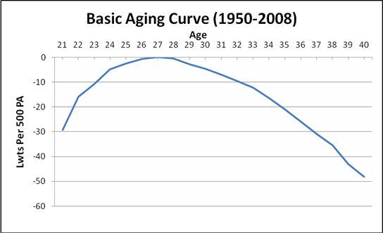
As you can see, the peak age is 27-28 (more of a plateau from 26 to 28). After that there is a gradual decline of around two to three runs a year until age 33, then a steeper decline (four to five runs a year) until age 38, after which the decline is steeper still.

Comparing Eras (pre and post-1980)

There has been some suggestion in the research that the aging curve is substantially different in the modern era, due to advances in medicine, higher salaries, and perhaps PED use. Let’s split the data up into two arbitrary eras, pre- and post-1980.

Table II: Average change in offensive performance from one age to the next (1950-1979)

                          Average
    Age                   Change   Cumulative
  Couplet      Players    in LW    Difference
   20/21         115       -7.7      -29.6
   21/22         226       14.4      -15.2
   22/23         398        5.6       -9.6
   23/24         588        6.3       -3.3
   24/25         783        1.7       -1.6
   25/26         880        1.4       -0.2
   26/27         868        0.2        0.0
   27/28         852       -0.5       -0.5
   28/29         793       -2.0       -2.5
   29/30         711       -3.3       -5.8
   30/31         627       -2.3       -8.1
   31/32         538       -2.6      -10.7
   32/33         426       -3.4      -14.1
   33/34         342       -4.9      -19.0
   34/35         272       -5.1      -24.1
   35/36         189       -8.0      -32.1
   36/37         124       -8.6      -40.7
   37/38          79       -5.7      -46.4
   38/39          55      -11.7      -58.1
   39/40          31       -1.5      -59.5

Table III: Average change in offensive performance from one age to the next (1980-2008)

                          Average
    Age                   Change   Cumulative
  Couplet      Players    in LW    Difference
   20/21          27      18.4      -27.1
   21/22         140       9.4      -17.7
   22/23         329       4.6      -13.1
   23/24         636       6.0       -7.1
   24/25         993       3.0       -4.1
   25/26        1224       2.4       -1.7
   26/27        1272       1.5       -0.2
   27/28        1236       0.2        0.0
   28/29        1160      -2.0       -2.0
   29/30        1064      -0.4       -2.4
   30/31         956      -2.0       -4.4
   31/32         819      -1.8       -6.2
   32/33         716      -1.7       -7.9
   33/34         581      -3.1      -11.0
   34/35         461      -3.7      -14.7
   35/36         358      -3.0      -17.7
   36/37         266      -3.4      -21.1
   37/38         183      -4.0      -25.1
   38/39         116      -5.9      -31.0
   39/40          70      -5.9      -36.9

Chart II: Comparing the aging curve in two eras (1950-1979 and 1980-2009)

Indeed, in the 1908-2008 era, peak age is a little later (28 versus 27) and the decline after that is significantly more gradual. Today’s 35 is the equivalent of yesterday’s 33, and players at 40 in the modern era are more productive than those at 37 prior to 1980. As you can also see from tables II and III above, there are many more players in their 30s in the post-1980 era.

That’s a pretty straightforward and unsurprising conclusion. Unfortunately, there are issues with this approach, as there always are in baseball analysis. In my next article, I’ll take a particular look at the issue of “survivor bias” and modify my approach in response.