The Physics of Fielding Grounders
Fielding ground balls is reactionary, but there’s a lot of science that goes into actually making the play. (via Paul L. Dineen)
I have often said ballplayers are pretty good experimental physicists. It turns out infielders specifically are also excellent at geometry, especially the geometry of triangles. So, let’s take a look at the challenge of collecting grounders from this point of view. We might even learn a thing or two that could possibly improve infield shifts.
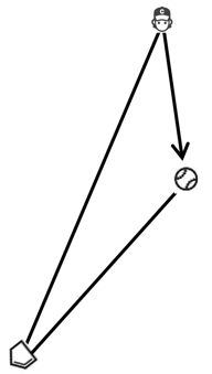
On every ground ball, infielders need to solve the triangle shown below. One side goes from home plate to the original position of the infielder. The second side goes from home to the location of the ball, and the final side goes from the initial position of the fielder to the ball.
The solution to this triangle is complicated because the sides that involve the ball change their length as the ball moves toward the outfield. The infielder has to move the right direction so his path intersects with the moving ball. In addition, the fielder would prefer to get to the ball as quickly as possible to improve the odds his throw will beat the runner at first base.
The infielder has the choice of directions. The sketch below shows five of the infinite number of possible routes to the ball, labeled a through e. The ball has traveled for less time to get to point a than to point b, and so on for each point. Meanwhile, the distance the fielder has to travel drops from point a until point c. Then distance begins to grow again if he chooses to move to point d or e.

So, a graph of the distance the fielder would have to travel versus the time the ball has traveled would look something like this.

The exact shape of the graph depends upon the speed of the ball, the initial position of the fielder, and the angle between the path of the ball and the initial direction to the infielder. Since these values aren’t known at this point, there is no scale on either axis.
Don’t be confused into thinking the infielder can necessarily get to the ball at point a, or b, or even c. That depends upon the speed of the infielder as well as the parameters that determine the exact shape of the blue curve described in the previous paragraph. Below are four such curves that vary due to changes in the speed of the ball.

The lowest spot on each curve is point c (where the direction of the ball is closest to the original spot of the fielder) for a ball with the given speed. The ball is moving the fastest for the red curve and the slowest for the blue curve. You can see this because the ball reaches point c at different times.
So, the next thing we need to think about is the motion of the fielder. Here’s where I have to come clean. I will use an overly simplified description of the motion of the fielder just to get some of the main ideas across. I have included in the appendix all the thorny mathematics for a more realistic motion of the fielder and the ball.
Your call. You can go directly to the appendix and enjoy a mathematical treat or you can stay here and be more comfortable. I suppose you don’t have to choose one or the other. You could do both, but if you do so, you probably are not destined to become an umpire. You would have to pick either out or safe – there’s no middle ground.
The simplest possible model for the motion of the fielder assumes the fielder moves at a constant speed from the moment the ball is hit until it is fielded. Yes, I know this is silly, but it has two virtues: It is easier to understand than more realistic models, and it will give some important insights. So, please play along or just go to the appendix.
A fielder moving at a constant speed would cover equal distances in equal times. This is equivalent to adding a straight line in the graph above. The larger the slope of the line, the faster the fielder is moving. The black line in the graph below is the motion of the fielder.
In addition to the straight line, I have included curves for balls traveling at four different speeds. The colored curves intersect with the black line at the shortest and longest times for the fielder to reach the ball.
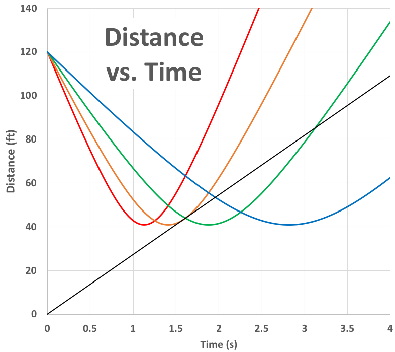
The blue curve illustrates the situation where the ball is moving slowly. So, the infielder must charge the ball and cover a lot of distance to get to the ball as soon as possible. Here is an example of such a play.

Nolan Arenado used his quickness to get to the ball near point b and meet the ball just as it gets there. Instead, he could have could have run more slowly to point e to field the ball, but by the time the ball made it there, the runner would have been safe.
The fielder could go to any point on the blue curve past the intersection with the black line and still get the ball because the black line only crosses the blue curve one time. However, as you just saw, the runner likely would be happily enjoying his infield single unless the infielder gets to the ball near the intersection of the blue and black lines.
The green curve expresses the situation where the ball is moving a bit faster than the blue curve. For the blue curve, the fielder could run to any point and get the ball, but here he only has the freedom to field the ball between the two intersections of the green curve and the black line. Again, the fielder would prefer to get the ball closer to the first intersection to minimize the time.
This video demonstrates such a play. It is called a “routine grounder.” It is hard to find a video of such a common play, so you’ll have to settle for the start of this double play.
The orange curve shows the situation where the ball is moving a bit faster still. Notice the infielder has to almost back away from the plate to field the ball because the intersection is past the bottom of the curve (point c). There is only one precise path the fielder can take to catch the ball because the orange curve interests the black line at only one place. Francisco Lindor seems to be a fixture on the highlight reel with these types of plays.
Finally, there is the red curve. In this case, the ball is moving so quickly compared to the infielder that there is no intersection between the red curve and the black line. That is, there is no way the fielder can get to the ball. You’ve seen this happen a million times. It is called a “solid single.”
So, despite the fact that this model is way over-simplified, it demonstrates the types of plays an infielder must make: charging a slow dribbler, the routine grounder, diving for a hot smash, and watching the ball find a hole. In addition, there may be some implications that might inform defense shifts. Most shifts are based on just the direction the batter usually hits the ball. However, the speed of the ball may be associated with these directions.
For example, consider a shift with three defenders on the right side against left-handed pull hitter who hits the ball harder near the right-field line and hits it slower up the middle. The shift might be more effective if the middle fielder on the right side sets up closer to first than to second, cutting down the angle for the balls moving faster.
Major league infielders are indeed masters of the triangle. If you are masochistic enough to want to see the mathematical details, read on, my friends.
Appendix
The triangle we need to deal with is shown below. The line between the plate and the initial position of the infielder has a length r. The line between the plate and the spot where the ball is fielded has a length db. The line the fielder travels to get the ball has a length df. The angle between r and db is labeled θ while the angle the between r and df is called φ.

For now, we need a relationship between the three distances given by the Law of Cosines,
Note that df and db depend upon the time since the ball was struck. You can choose whatever model you like for those quantities. My preference for the fielder distance, df, is the simplified sprinter equation, where the fielder starts at rest and speeds up to a maximum value,
![]()
where vt is the top speed of the fielder, and c which sets the rate at which the fielder’s speed increases.
My choice for the motion of the ball is one that slows exponentially,
![]()
where vo is the initial speed of the ball, and k describes the rate at which the ball slows down.
The Law of Cosines gives the following mess,

Choosing values for the six parameters r, θ, vt, c, vo, and k allows the equation above to be solved for the times when the curves intersect. The solution likely needs to be accomplished numerically.
In the limited time I had to fiddle around with the solutions, I found there is always a solution with a negative value for the time. You can ignore this solution unless you believe somehow you can go back in time!
There are as many as three positive time values. The third value comes about because the right side of the parabolic curve is driven back downward by the slowing of the ball, especially if the ball slows rapidly.
You can find df and db by plugging in the times you just found into the equations above. You can then go on to find φ if you like using the Law of Sines,

Well, go get on it. Improve those defensive shifts.
OK, this is really cool. The time an infielder takes to get to a ball, at least for me, is about reading the hops… it’s really the most important thing I take into account on my route. For “routine” groundballs, or ones I have to charge, getting the short hop or long hop is key.
That’s absolutely a part of an infielder’s calculation. In some ways, what hop you get is even more important than the intersection. Not only does the hop dictate your ability to glove the ball, but it also impacts the footwork behind a throw.
love these articles, as both physics undergrad & shortstop. another variable to contend with is the angle relative to first base the infielder will be at when fielding the ball, which is dependent on the path taken, as that affects throwing mechanics. if we imagine a line extending through the infielder’s shoulders being intersected by a line from first base and consider the angle created between the “shoulder-line” and first base as typically being behind first base, the angle is preferably close to zero or 360 degrees, assuming the line extends only from the infielder’s left (non-throwing) shoulder. an angle close to 180 degrees– i.e. if a shortstop has to towards 2nd base to snare a grounder is more difficult to throw from, as it necessitates either a counterclockwise spin and throw or a resetting of the feet from a dive. both are possible, but do take more time and are maybe not quite as accurate. perhaps that’s why shortstops have the most diverse range of throwing motions, to enable them to catch balls at all kinds of angles and directions of momentums and still be able to get the out.
outfielders use triangles too, in a slightly different way. the most efficient routes necessitate estimating where a ball will land and then taking the most direct route to a place where the ball is at a catchable height, if they can get there in time. corner outfielders often have to include the fact that the ball can be slicing away from them, too.