Building a Robot Umpire with Deep Learning HD Video Analysis (Part Three)

Anything that can be done to improve umpires is a good thing. (via Mark Mauno)
This article is a continuation of my previous articles here and here. In this article, I will discuss additional improvements to my robot umpire system, the most prominent of which is using HD source video.
HD Video Background
HDTV (high-definition television) started broadcasting in the 1990s. Perhaps not surprisingly, live sports was one of the main selling points that convinced people to spend thousands of dollars on a new television set that could only receive a handful of HD broadcasts (if you were lucky). MLB was the first North American professional sports league to air a game in HD, broadcasting the Opening Day game between the Rangers and the White Sox in 1998. Twenty-one years later, in the year 2019, you will be hard pressed to find any live sports broadcast that is not shown in HD.
HD sports broadcasts typically have a resolution of 1280×720, which is usually called “720p.” This is several times the resolution of SDTV (standard definition television) and many more times the resolution of the old analog television broadcasts. The next generation of broadcast video is commonly called “4K,” which, at a resolution of 3840×2160 pixels, has many times the resolution of HD video. While DIRECTV and Rogers are now broadcasting a handful of games a year in 4K, the vast majority of people in North America are still watching baseball in HD.
The Ups and Downs of Higher Resolutions
The HD source videos used for my analysis were 720p at 30 fps (frames per second), while the first two parts were done on 360p videos (with a resolution of 640×360). Thus, these HD videos have four times the number of pixels, with twice the number of pixels in each of the horizontal and vertical dimensions. This is important for us, because with four times the pixels, all the objects in the video (including the players, home plate, and the ball) appear much larger. So if we can harness these videos properly, we expect we should be able to build a better robot umpire.
However, there is one big issue. Recall that I extracted the features from the video frames with the Inception V3 convolutional neural network. Inception V3 operates on image patches of size 299×299. Because the previous videos were low enough in resolution, I was able to simply crop out a fixed window in the “middle” of each frame, and I would always be guaranteed the cropped section would contain the batter, catcher, home plate, and the ball (all of which are necessary in order for the system to be able to determine if the pitch is a strike or a ball). With these new HD videos, this is no longer possible.
Below I show two screenshots from two different games, each with a 299×299 patch containing the batter, catcher, and home plate highlighted in yellow. You can clearly see these highlighted windows are in different positions. This is partially because one batter is a righty and one is a lefty and partially because the camera viewpoints are different. Since successive batters often will alternate between righties and lefties, the proper window will change many times even within a single game. Therefore, it is just not possible to pick a fixed window to crop.
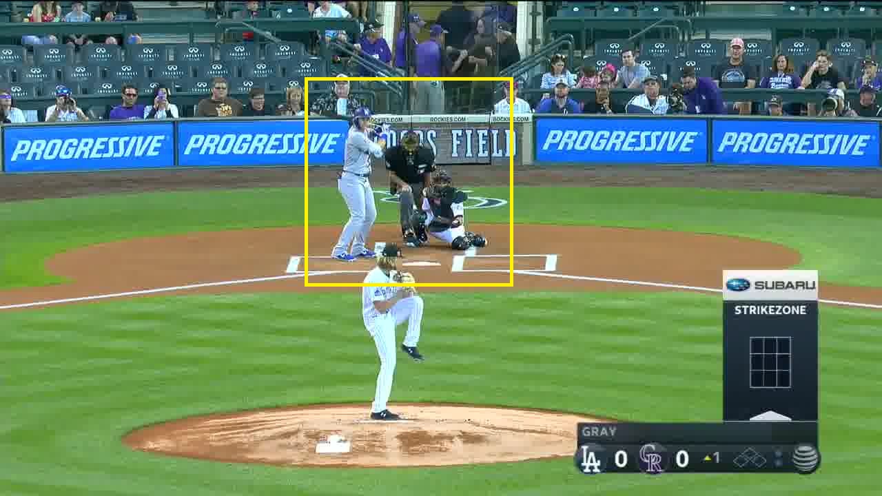
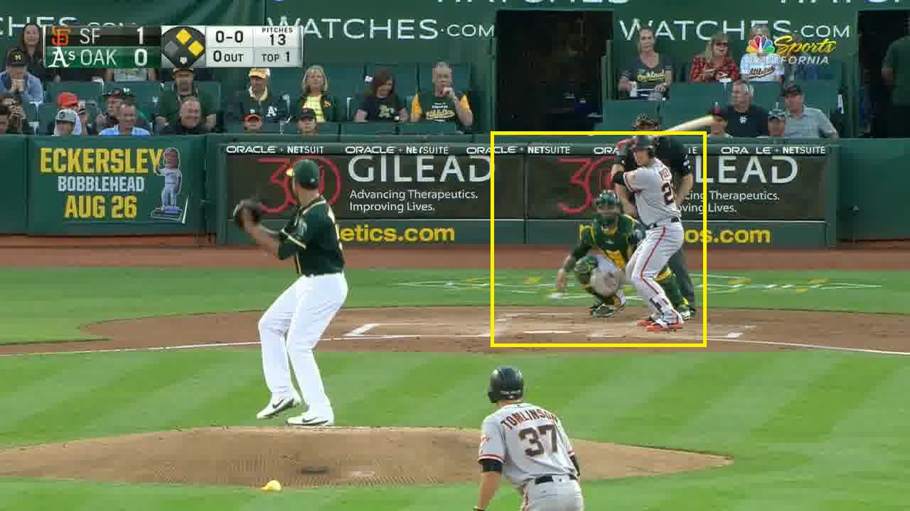
There are two solutions to this problem. One solution is to crop multiple 299×299 windows per video frame. It seems reasonable that two 299×299 windows horizontally side-by-side should be enough to guarantee you capture all the necessary objects. A second solution is to try to determine where within the frame the objects are. I chose to use this approach.
Finding Home Plate, the Catcher, the Batter, and the Ball
Fortunately for us, object detection is one of the most common use cases of deep learning, and once again, we can leverage existing work and use a model that is specifically trained for object detection. Tensorflow comes with a whole bunch of object detection models here. These models are trained to detect a certain standard set of objects. One such set of objects is COCO (Common Objects in Context). If you browse through the COCO website, you will see — as our luck would have it — the set of objects includes baseballs, baseball gloves, and baseball bats.
It seems natural for our first instinct to tell us to use the model to find where the ball, gloves, and bat are in the image. Unfortunately, this won’t work very well. All three of these objects are quite small compared to the context of the rest of the image. Whereas the whole image is 1280×720, a ball may have a size of 10×10, which is 1/1000th the size of the whole image. Not only will the model have a hard time finding the ball, it will also mistakenly label other round objects as balls, which is troublesome. Gloves are larger than balls, but they are still small relative to the whole image and thus also have the same problem. Bats are much longer objects than balls or gloves, but in my experimental results, in the majority of cases, the model could not identify the bat with confidence.
So what can the object detection models detect with confidence? Players! The players are typically the largest objects in the images, and the models are trained to detect people (which is perhaps the most common use of object detection). Here is the result of running the model on an image.
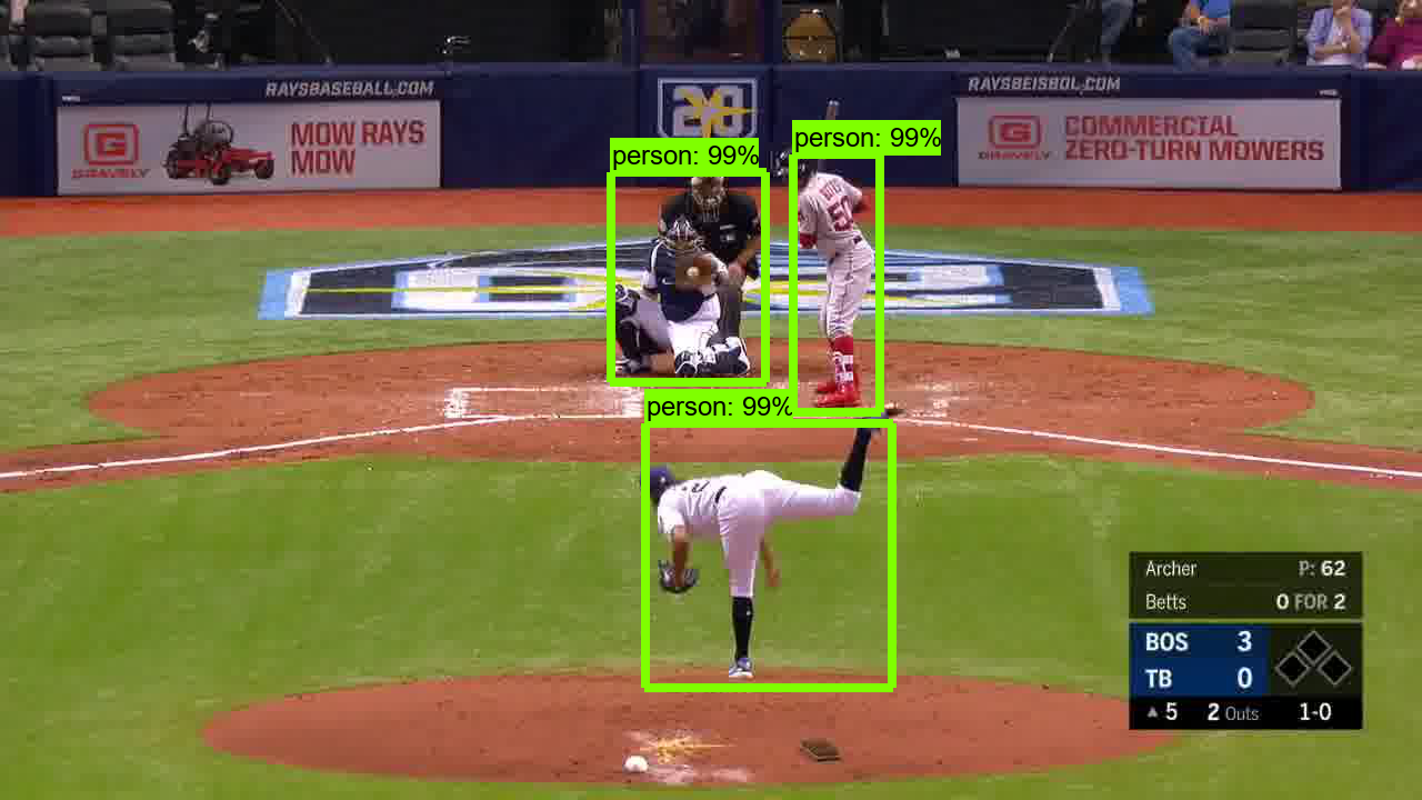
The pitcher, batter, and catcher are all detected with 99 percent confidence. There were other objects detected, too, with less confidence, but I filtered those out. Note that there is a tradeoff between detection confidence and speed. More complex models will yield more confident detection results but will take more time to execute per image. We have our choice of many models, and it is up to us to determine what is the most appropriate model for this job. I wound up picking the “faster_rcnn_resnet101_coco” model, which yields good confidence at detecting players while executing each frame in an average of 89 milliseconds.
Now, how do we go from here to determining where home plate is? Basically, in my program, I would parse the detected results and try to find “two people near the center of the image standing close to each other without significantly overlapping each other.” To determine which person is the batter and which is the catcher, I assumed the catcher has a higher lower-boundary y-coordinate, since his feet are situated further up in the image than the batter’s feet. Armed with these coordinates, I finally can crop out the appropriate home plate region.
Note that this process is not foolproof. Sometimes in the first frame, the batter and catcher will not both be detected, so I often had to try multiple successive frames until getting a match. Sometimes the umpire will be detected, which can throw off my result parsing logic. Sometimes the players are detected but the detected coordinates are slightly shifted, which can result in either the batter or catcher getting partially chopped off in the final cropped region. All of these sporadic issues are okay; I manually inspected samples of the final set of cropped images, and I determined the images as a whole had high enough fidelity for the job.
Using Mirror Images to Get More Training Data
As I’ve alluded to in previous articles, all deep-learning models benefit from having more clean training data. One way to get more training data for our task is to process more pitch videos. Compared to Part 2, I expanded my data set to include videos from the 2012 to 2018 seasons. This was all the HD videos I could get at the time, so to go further, I resorted to using a common trick, to take the mirror image of the images.

Here is a sample cropped image.
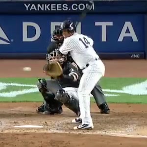
Here is the same image flipped around.
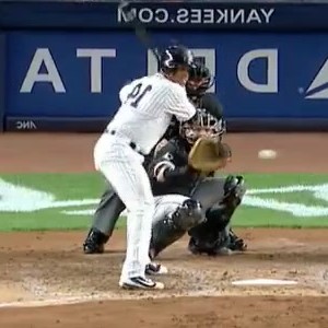
Whereas the original image is of a right-handed batter, the flipped mirror image can be credibly thought of as an image of a left-handed batter. The words “YANKEES.COM” and “DELTA” are now flipped around and reversed, but the classification algorithm doesn’t care about words in the images (or really, about anything in the background). To the algorithm, this image is basically as good as the original one for training the model.
The main drawback of using these mirror images is that we are implicitly assuming the strike zone is identical for righties and lefties, which in theory should be true but in practice is not exactly the case. If we were trying to match or exceed the performance of a human umpire, this could be an issue. However, given that in the previous articles we were doing quite a bit worse than a human expert umpire, I suspect this additional data certainly will help improve our results.
Note that these mirror images are only used in the training phase, they are not used in the validation and testing phase. When we validate and test the model, we only want to use the original images to measure the fidelity of the model.
Training, Validating, and Testing the Model, and Tuning the Hyperparameters
The total data set totaled over 3.2 million samples. Just like before, the cropped images were fed into an optical flow calculation program, and then both the RGB image and the optical flow image were fed into the Inception V3 CNN in order to generate a 4096-element feature vector. Then these feature vectors were fed into a LSTM RNN, also like before. However, this time around I spent much more time on model validation and hyperparameter tuning. In particular:
- Instead of splitting the data into separate training and test sets, I now split into training, validation, and test sets.
- Instead of just a few days, I spent almost two months searching for the best model hyperparameters.
My previous data split was 80/20 training/test. This is a traditional split that makes sense when you have thousands or tens of thousands of data samples. However, in the age of big data, when you have millions of data samples, it is often no longer necessary to devote 20 percent of the data to test purposes. The purpose of the test set is to check how well the model will do on new data. Research has shown that you don’t need millions of samples to fulfill that goal; usually tens of thousands is enough. Therefore, I decided to use 95 percent of the data in the training phase, which is common with data sets of this size.
The validation phase is designed to determine the performance of each model with a specific set of hyperparameters. I chose to search for the best hyperparameters by randomly generating hyperparameter values within some set bounds. Perhaps somewhat surprisingly, this method is used relatively often in academia and industry. Once we find a model that gives us the best performance in the validation phase, we measure it’s performance on the test data set to get the final performance. This is done to avoid overfitting to the validation data set, and it gives us more confidence on the model’s performance on new data. Of the five percent data that was not used in the training phase, I divided it evenly to form the validation and test sets, so each set has 2.5 percent of the overall data.
Results
Here are the graphs of ROC and F1 score vs. Ball/Strike Threshold.
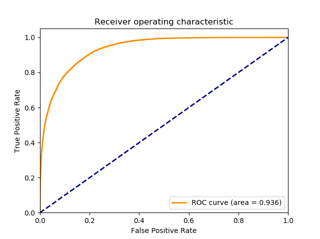
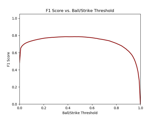
You can see immediately the results are improved compared to Part 2. The ROC curve has a much larger “hump,” and the F1 score curve is much flatter than before and thus yields a similar F1 score over a much wider range of thresholds.
Here is the confusion matrix of the test set data, with the ball/strike threshold set at 0.39 to optimize for maximum F1 score.
| Deep Learning’s call (down) / Umpire’s call (right) | Strike | Ball |
|---|---|---|
| Strike | 19057 | 6225 |
| Ball | 4125 | 44625 |
Here is a comparison of the current robot umpire’s performance against the previous robot umpire performance and the human expert (aka, myself) performance.
| F1 score | AUC | |
|---|---|---|
| Robot Umpire – Part 2 | 0.673 | 0.850 |
| Robot Umpire – Part 3 | 0.786 | 0.936 |
| Human Expert Umpire | 0.871 | — |
We have taken a large step towards approaching human expert performance. Our performance certainly has improved over the result in Part 2, although you should keep in mind that Part 2 only used four years of video data instead of seven years in Part 3, so it’s not exactly an apples-to-apples comparison. Note the AUC is not defined for the human expert, because a human will only make discrete ball/strike calls instead of assigning a probability for each event.
Conclusion:
In Part 3 of this project, we successfully utilized HD-resolution video in our quest to build an improved robot umpire. There are additional pre-processing steps necessary when dealing with HD video, but the improved results more than justify the extra effort required.
Daren Willman of MLB tweeted recently that videos for all pitches since the 2018 season are now available for download on https://baseballsavant.mlb.com. While it used to be a fairly tedious task to collect video data for a project like this, easy public access to these videos makes it possible for everyone to get their feet wet. I bet many of you readers can do a great job in building a robot umpire if you put your minds to it!