The Math of Weighting Past Results
The 2016 season has just ended. You’re the GM of your favorite team, and your team needs a center fielder (if you’re an Angels fan, you’ll have to pretend you’re somebody else’s GM for this exercise). You’ve got two names in front of you: Dexter Fowler and Carlos Gomez.
Whom do you offer more money? Both are around the same age. Over the past three years, they’ve put up pretty similar value (9.5 fWAR for Fowler vs 9.2 fWAR for Gomez). Fowler’s been the better hitter and Gomez the better fielder, but overall, they’ve been pretty similar.
The actual MLB GMs gave a pretty clear answer to this question. Fowler signed for five years and $82.5M, while Gomez signed for one year and $11.5M. Why the disparity? Recency. Fowler was coming off the best season of his career, while Gomez was coming off a season during which he got released by the Astros. And while Gomez has rebounded fairly well with the Rangers, Fowler was easily the better bet coming into this season.
The same reasoning is why projection systems give more weight to more recent seasons. Whenever teams’ or players’ talent levels are constantly changing, recent data tell us more about their current talent than older data.
Weighting is most commonly done by season, but the same concept applies within a single season as well: If you break a player’s season down day by day, the past few days will tell you more about his current talent than an equivalent amount of data from the beginning of the year.
Weighting Past Results
Weighting day by day requires far more individual weights than weighting by year. As a result, it is usually impractical to determine each weight individually. Instead, day-to-day weighting usually relies on fitting an exponential decay factor to the data rather than individually tuning each weight. The basic formula for determining how much weight to give data from a given day under this model is:

If your decay factor is .999, then each day further back will get 99.9 percent the weight of the following day. It should be noted that exponential decay is not necessarily implied by the mathematical processes of talent changes—it’s simply an assumption that makes calculating the weights much simpler. It does, however, provide a good fit for the true weights of simulated data, so using it should not cause any problems.
Before we go further into day-to-day weighting, let’s start with a simple example using team seasons to see how weighting past data works. In our example, each team will have a fixed talent level for a given season, but that talent can change from one season to the next. We’ll say the variance in true-talent winning percentage across the league is 0.0036 (which is approximately what it is in MLB), and the correlation of true-talent winning percentage from one year to the next is 0.9.
I’ve simulated two seasons for a bunch of teams under these conditions. Because we’re only dealing with two seasons, we don’t need to worry about exponential decay and can just focus on how to weight one season relative to the other.
Now, say we want to estimate each team’s talent level in the most recent season from the results of the sim. We can test various weights for year one to see what mix of Years One and Two gives us the strongest relationship to talent in Year Two.
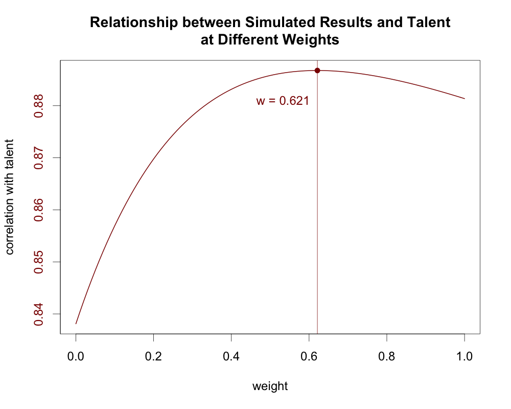
The correlation between results and talent peaks when the first year gets about 62 percent the weight of the second year. Similarly, if we run a linear regression using the results from Years One and Two to predict talent in Year Two, the first season gets about 0.62 times the weight of the second season:
When talent levels are changing, older data contains more random noise than recent data: You not only have the random noise from sampling error, but also from the changes in talent that build up over time. By reducing the weight of this less reliable data, we diminish that noise.
If we keep reducing the weight of old data, though, we eventually hit a point where we start throwing out more useful information than random noise, and going any further starts to make our estimate worse. In our simulated example, that happens at a weight of 0.621.
Weight too aggressively, and you end up discarding too much of the valuable information held in past data. Weight too leniently, and you give too much impact to the random noise introduced by talent changes over time. The trick with weighting is to find the point where these factors balance out.
General Principle No. 1
Weighting past results is a balancing act between diminishing the random noise from talent changes while keeping as much signal as possible from past results. The proper weighting that balances these factors will maximize the relationship between observed results and talent.
Another Example
Now, let’s repeat our simulation, but instead of two 162-game seasons, we’ll just simulate two games for each team, with talent changing between games.
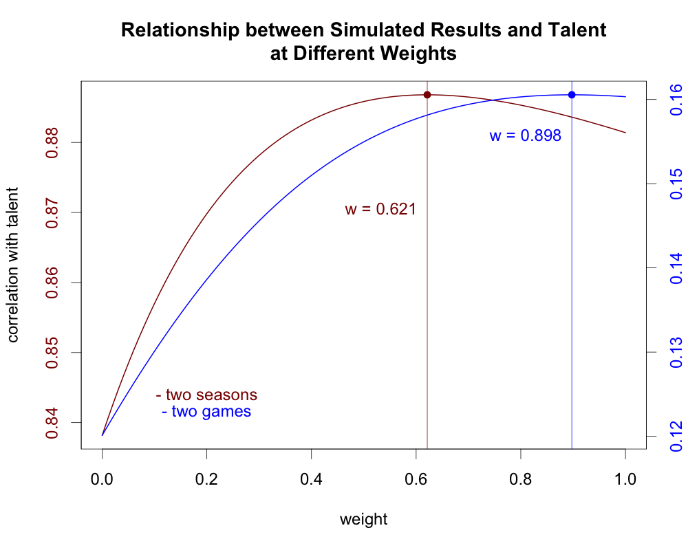
Everything in these two scenarios is the same except for the number of games played at each talent level, but here the ideal weighting jumps from 0.621 to 0.898. Furthermore, in the latter scenario, there is barely any difference between using the ideal weighting and not weighting at all.
This example comes from a discussion the Tangotiger blog where the idea of having a decay factor equal to the golden ratio (approximately 0.618) came up. Because of how the golden ratio works, the weight of one day by itself will equal the combined weight of the two days before it. (There is a reason I only simulated two days rather than three, but we’ll get into that later.)
Jared Cross responded in that thread showing that you get a weight of 0.618 for the previous day when the day-to-day correlation for a team’s true talent winning percentage is about 0.6234. More interestingly, he also found that if we assume teams have a fixed talent level for a full season and that talent only changes from one season to the next rather than each day to the next, then we’d need to raise the year-to-year correlation of talent to 0.897 to get the same weighting.
In the examples above, I kept the correlation of talent constant and let the weighting change, whereas Cross kept the weighting the same and changed the correlation of talent, but both illustrate the same point: The ideal weighting depends not only on how talent changes from day to day, but also on how much data you have.
To paraphrase Cross’ explanation, this happens because a 162-game sample tells us more about a team’s underlying talent than a one-game sample. Because we know more about each team’s talent level from our recent data alone, we can more easily discard past data with a more aggressive weighting.
Think about it like this: Say you had a million observations for each player at their current talent levels. The million observations would tell you almost exactly what each player’s current underlying talent is, so you’d have no reason to bother looking at any older data from previous talent levels. Including the outdated data would just pollute your estimate of current talent by taking your near-perfect estimate and moving it toward the player’s previous talent levels.
On the other hand, If you only had one observation from the current talent level, that one observation by itself will tell you very little about the current underlying talent levels. You need to look at older data to even get a general idea of each player’s talent level, so you can’t be so quick to discard that data.
In other words, how much you know about the underlying talent levels is one of the factors that affect the balance between preserving the signal versus discarding the noise that older data introduces. The more you already know, the less you need to preserve the noisier signal from older data.
General Principle No. 2
Weighting depends partially on how much talent changes from day to day, but it also depends on how much you can tell about the underlying talent levels from your data. In general, the more your recent observations tell you about the underlying talent levels, or the more data you have, the more aggressively you can discount past results.
Factors That Affect Weighting
I’ve talked a little bit about day-to-day weighting versus year-to-year weighting, but what is the actual difference between the two? Essentially, day-to-day weighting requires cutting your data into more pieces, and each individual piece contains much less information. Fundamentally, though, there isn’t really any mathematical difference between weighting day to day versus year to year.
In our two examples, the reason the weighting changed so drastically was solely because in the former we had 162 observations at each talent level, while in the latter we had only one. The fact that one used seasonal data and the other used day-to-day data has nothing to do with it beyond the amount of data used.
If, for example, we wanted to look at a team’s swing percentage instead of its winning percentage, it would be completely reasonable for a team to face 162 pitches in one day, and that example would behave more like the two-season example than the two-game example even though it is also day-to-day.
This applies to any length of time. As long as your data is broken into consistent intervals, it doesn’t matter how much actual time passes in between. If you want to look at fastball velocity for starting pitchers, you don’t have to worry about the fact that there are four rest days in between each start. You can just treat each start as one unit of time and go from there. For the remainder of this article, I will simply refer to “day-to-day” talent changes for simplicity’s sake, but keep in mind that “day-to-day” can be whatever unit of time is appropriate.
So the actual unit of time between each talent change isn’t important as long as we are dealing with consistent intervals. The amount of data we have, however, is important, and, more generally, anything that affects how much we know about the underlying talent levels is important.
Mathematically, the idea of “How much do we know about underlying talent levels?” can be expressed as the proportion of overall variance that can be attributed to the spread in talent across the league. In other words, how much of our observed data comes from the differences in talent between players as opposed to random variance or other factors unrelated to talent?
This was an important theme in my previous article on how changing talent levels affect variance, so I won’t go too deeply into that here, but the basic idea in terms of player projections is this: The more of your observed variance that comes from the spread in talent rather than other factors like sampling error, the more likely each player’s past results will carry forward into their future results.
This gives us two specific values that will affect weighting: the observed variance in your sample, and the variance in talent across the population. This also means anything that affects the observed variance, like the number of observations you have, will have an impact on weighting as well.
If we go deeper into the math behind weighting, we will find that there are actually just four values that determine the proper decay factor for a given data set:
- The variance of current talent levels in the population.
- The observed variance for one day’s worth of results in your sample.
- How much talent changes from day to day (as measured by the correlation of talent from one day to the next).
- How many days are in your sample.
That’s it. And technically, you don’t even need to know the variance in talent and the observed variance separately since only the ratio of those two values matters, but it’s not really any easier to find the ratio than to just find the values themselves.
That fourth factor, by the way, is why I made sure to simulate only two days instead of three in the example stemming from the golden ratio discussion. If I had used three days instead of two, it would have changed the weighting so that the decay factor no longer matched with what Cross got.
General Principle No. 3
The decay factor used to weight past data for a given data set depends on the four factors listed above. Each of these values is related to how much your data tells you about the underlying talent levels, which in turn determines how to balance the mix of signal and noise in past data. As long as you have these four values, other factors, including the actual length of time for each unit of data, are inconsequential to weighting.
Why Not Linear Regression?
Before we go forward with our model for estimating the decay factor, let’s take a minute to address the statistical elephant in the room: Why can’t we just use a linear regression to estimate the weights used to discount past data?
Linear regression generally works fine for determining how to weight past results if you are working with seasonal data, as many projection systems do, but it can run into some serious issues at the day-to-day level. With seasonal data, we are dealing with at most a handful of variables (each separate season), and each variable in the regression contains enough data to be a reasonably reliable indicator of talent.
With day-to-day data, we suddenly have a hundred or more variables, and each of them is swamped with random variation. This leads to overfitting, which is when your model has so much data relative to that data’s usefulness that it is easier for the model to cherry pick a pattern out of randomness than to find any actual relationship to the underlying probabilities.
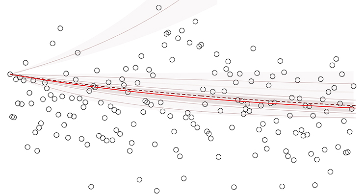
As an example, I’ve simulated 10,000 full player-seasons (four plate appearances per game over 162 games) of on-base percentage data and then run a linear regression to assign weights to each of the first 161 games to predict the results from the 162nd game. For comparison, I’ve included the proper weights (dashed dark red line) along with an exponential decay function best-fit to the regression coefficients (solid red line).
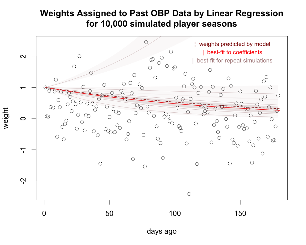
The coefficients are all over the place with no clear pattern. They should all fall between one (data from that day gets full weight) and zero (data from that day gets no weight), but the regression assigns weights well outside that range. And, while the best-fit line for the coefficients isn’t that far off what it should be, repeat simulations show that is just random luck. Ten thousand player-seasons is huge in terms of actual MLB data, but it’s still not nearly enough when we’re dealing with data this granular.
Averaging the results of a linear regression to get an overall trend is also tricky. Our exponential model means we expect a constant ratio between the weights given to any two consecutive days, but if we just take all the ratios of consecutive coefficients from the regression and average them, we’ll invariably get something too high. The average ratio from the above graph is 1.05, for example, which would mean data gets more weight the older it is. (This is a mathematical artifact from how averaging ratios works when there is uncertainty in the denominator as well as the numerator.)
You basically need to best-fit another equation to the coefficients if you want to average your results to find an overall trend. This isn’t necessarily a problem as long as whatever software you use to run the linear regression can also best fit an exponential function, but it’s an issue you need to be aware of and another step in the process.
That said, linear regression can work well if each individual unit of data has enough information to give you reliable results, which is why it typically works better for seasonal data. Even if that is the case, though, it will still be useful to develop a more general model for weighting.
This is because the proper weighting depends on how much data you have in your sample. Even when you can use linear regression effectively, you’d have to run a separate regression to generate new weights each time you wanted to apply them to a different size sample. Having a model to translate your results to varying samples would simplify this process and give you more consistent results.
As a side note, in cases where you can use linear regression effectively, you can actually use the weights given by the regression to estimate the correlation for changes in talent (which, as we saw in the previous article on variance, can be difficult to estimate).
General Principle No. 4
Linear regressions are generally not that useful for estimating the proper weighting at the day-to-day level. They are better suited for seasonal data, where you have fewer variables and each data point has a stronger relationship with the underlying talent levels.
Developing a Model for Weighting
One of the key concepts from the previous article was the close relationship between correlation and variance in describing how well observed results project talent levels. This will be useful here as well, where we are trying to maximize the correlation between weighted results and current talent.
The relationship between correlation and variance is defined by the following formula, where Cov is covariance and sd—standard deviation—is the square root of variance.
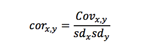
Using this formula, we can calculate expected values that match the graph from our earlier simulated examples where we mapped correlations to various weights. To do this, we need to know three values: the variance in current talent levels (our y variable), the variance in weighted results (our x variable), and covariance between current talent and weighted results.
Some Math: Calculating the Variance and Covariance
Variance in True Talent
The variance in talent can be estimated using the methods discussed or linked in the previous article on variance, so I won’t go over it here, but there is one important thing to note. That article concluded that the variance in talent tends to shrink as your sample grows whenever talent levels are changing. For this, you’ll want the variance for a single point in time rather than over your full sample since we’re estimating current talent.
Variance in Weighted Results
We can measure the variance of the weighted results directly, but it will be more useful to break that observed variance down into some more general factors so we can see exactly how each of those factors impacts the result.
When we compile our weighted results, we multiply the results from each individual day by the appropriate weight and then add those daily results together. We can think of each day’s results as a separate variable, so if we have n days of data, instead of one variable x, we really have n variables (x1,x2,…xn) added together.
When you add two variables, their combined variance will usually (though not always) increase, but by how much depends on how the variables are correlated. If the variables are uncorrelated, you just have to add the individual variances to get the combined variance. When the variables are correlated, though, you have to adjust the combined variance to account for that correlation. Combining large values with other large values (positive correlation) will exaggerate the spread of values, whereas combining large values with small values (negative correlation) will reduce the spread.
The general formula for finding the variance of the sum of two variables is:

If we have two days in our sample, x1 will be the set of results from Day 1, while x2 will be the set of results from Day 2. When we weight the results of Day 1 by a factor of w, this gives us:

There are a few tricks we can use to further manipulate this expression. First, Var(w*x1) = w2*Var(x1) and Cov(w*x1,x2) = w* Cov(x1,x2), so we can factor the w out of the variances. Second, our expected variance won’t change from day to day, so we can treat both variances as the same value. And third, the covariance term is equal to r*Vartrue, where r is the day-to-day correlation of talent and Vartrue is the variance in true talent.
(This last point has to do with the relationship between reliability, correlation, and, covariance, but in layman’s terms, you can think of the variance in true talent being the shared variance between the two days, and since talent changes between days, that shared variance is reduced by the amount talent changes.)

Covariance Between Weighted Results and Current Talent
Using the same logic of “shared” variance, the covariance between observed results and underlying talent is equal to the variance in talent. Again, this “shared” variance is reduced for the previous day due to the changes in talent.

By placing these three values into the formula for correlation, we get:

With a bit of simplification, this is equivalent to the following:
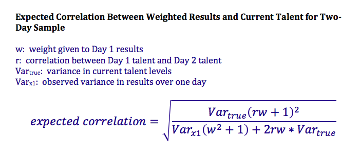
In order to find the proper weighting, we just need to find the value of w that maximizes this formula given our inputs for the other values (which is actually pretty difficult to do properly via calculus, but there are statistical programs, such as R, that have algorithms that can calculate this pretty easily).
To make sure this works as expected, we can compare the values from our earlier simulation to those predicted by the formulas. Using the two-season example from the beginning of the article and a weight of 0.621, we get the following values, where y represents true talent and x represents the weighted results:
| Formula | simulated | predicted |
|---|---|---|
| Vary | 94.7 | 94.5 |
| Varx | 292.0 | 292.3 |
| Covx,y | 147.5 | 147.5 |
| Corx,y | 0.8873 | 0.8870 |
Note the variances in this table are the variance in win totals and not winning percentage (because that’s how I happened to have the sim set up), but you can use either one.
Generalizing the Formula Beyond Two Days
This formula works for finding the proper weighting when you have exactly two days of data. Generalizing it to work for any number of days makes the math more complicated, but it follows the same basic principles.
I’ve gone through the math for generalizing this formula in a supplement on my blog for those interested, but here I’ll just go ahead and give the new formula:
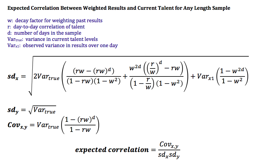
(As a reminder, “day” here can be whatever unit of time your data is divided into.)
Just as before, the decay factor is the value of w that maximizes the expected correlation. This is a fairly cumbersome equation to deal with, so I’ve included a calculator at the end of this article to make it more convenient to calculate.
We also can verify these formulas against simulated data. Using the simulated OBP data from the linear regression example and a decay factor of 0.9936 (which happens to be the ideal weighting for that dataset), we get the following:
| Formula | simulated | predicted |
|---|---|---|
| sdy | .120 | .122 |
| sdx | 14.5 | 14.6 |
| Covx,y | 1.34 | 1.37 |
| Corx,y | 0.770 | 0.771 |
General Principle No. 5
The formula to calculate the decay factor for a given data set is fairly complicated, but ultimately it depends on just the four inputs listed earlier. These inputs can be entered into the calculator below to determine the weighting for a given data set.
Difficulty Incorporating Past Years Into Day-to-Say Data
This article covers how to weight day-to-day data within a single season, or potentially year-to-year data from multiple seasons, but incorporating multiple seasons of day-to-day data runs into some difficulties.
This is because the math used here relies on the units of time representing consistent intervals in your data. Having large gaps between clumps of data throws off that math. The number of days in your sample is one of the factors in determining the proper weighting to use, but having 100 days worth of data from this season is different from having 50 days worth of data from this season and another 50 days from six months earlier.
Constructing a new decay factor that properly accounts for these gaps is not that simple. (If you followed the mathematical supplement I linked earlier, you’d have to alter the covariance matrix to account for the missing days, which complicates the rest of the math as well.)
It’s also possible that talent changes within a season are different from talent changes between seasons. The offseason is much different from in-season in terms of workouts, conditioning, wear and tear, and a player’s ability to experiment, so it makes sense that talent changes over 100 days in-season might be different from talent changes over 100 days in the offseason. I don’t know if this is actually an issue, but it would at least be worth studying.
I don’t have a good solution for this issue, but it is important to know this is a shortcoming of the calculator offered here. You might need to get creative in trying to adapt the weighting to cover offseason gaps, or you can just use the calculator as is and accept that it won’t be as accurate for this specific purpose.
General Principle No. 6
The math behind weighting past data gets more complicated when you introduce large irregularities in the gaps between your day-to-day results. Specifically, the offseason makes it more difficult to calculate an accurate decay factor for day-to-day data that covers multiple seasons.
Using the Calculator
To finish, let’s walk through an example of how to use the calculator using our OBP sim from the section on linear regression. Our variance in current talent levels is 0.0009 (sd = 0.030 points of OBP), the observed variance in OBP for each day is 0.0559 (which is approximately the random binomial variance over four PA plus the true talent variance), and the correlation of OBP talent from one day to the next is 0.998.
We simply plug these three values into the calculator, enter the number of days in our sample, and hit submit. If we have ten days, we end up with a decay factor of 0.99768. For 162, it’s .99389.
Alternatively, if you already know what the decay factor should be but don’t know the day-to-day correlation in talent, you can enter the other values and then guess and check to home in on the correlation that leads to the correct weighting. This could be useful if you are using year-to-year data instead of day-to-day data, where the decay factor is easier to estimate using linear regression. (My impression is that the decay factor we get in this example is fairly aggressive, so I probably picked too low a value for the day-to-day correlation in talent for the simulation.)
The weighting calculator should work for any type of statistic. If you are specifically using a binomial rate, I’ve also included an estimate of the regression constant to use for projecting current talent. After calculating the proper decay factor, just enter the league-average rate and the number of observations for each day.
(For the regression constant, you also need to make sure the variances you enter for the first step are variances in the binomial rate and not variances in number of successes (i.e. our standard deviation for talent is 0.030 points of OPB, not 0.12 times on base per four PA). You can use either scale for the weighting calculator as long as you use the same scale for both variances, but not for calculating the regression constant.)
I won’t go into the math for the regression constant since there is already plenty of math in this article (and I’m not completely confident I can explain it all that well), but we can test it against our simulated data. The league average in the sim was .330, and we had four PA per day. Over 162 days, that gives us a regression constant of 210, compared to 246 if we were to ignore changes in talent.
Now, if we project each player’s talent at the end of the sim and compare that to his actual talent level, we should find that, on average, the projections match up with actual talent. If the regression constant is too low, the projected talents will be further away from the mean than the actual talents. If it is too high, they will be closer to the mean.
After dividing the population into six roughly equal groups based on their projected OBP, here are the average errors in projected talent using regression constants of 210 and 246:
| Projected OBP | C=210 | C=246 |
|---|---|---|
| .352+ | 0.0008 | 0.0027 |
| .340-.352 | 0.0007 | 0.0016 |
| .330-.340 | 0.0004 | 0.0007 |
| .320-.330 | 0.0001 | -0.0002 |
| .308-.320 | -0.0004 | -0.0013 |
| .000-.308 | -0.0016 | -0.0036 |
The revised regression constant works better than the original regression constant for every group of players, and the original regression constant consistently over-regresses the results, indicating the original regression constant is too high.
Conclusions
Admittedly, this is a fairly mathematical article with some esoteric concepts, but there are still some important general takeaways. Perhaps the most important thing is that, when weighting past data, there is no one proper weighting intrinsic to each stat. The proper weighting depends on a variety of factors, and it can change depending on how much data you have.
Specifically, the four values that have an impact on weighting are:
- The variance of current talent levels in the population.
- The observed variance for one unit of time.
- The correlation of talent from one unit of time to the next.
- How many days (or other units of time) are in your sample.
Any time one of these factors changes, it will have an impact on the proper weighting required for your data set.
It’s also important to note that weighting impacts the regression constant, which I hinted at in another previous article. Weighting reduces your effective sample size in order to minimize the impact of variance introduced by changes in talent over time, and in doing so, it distorts the variances that form the basis of the regression constant.
There are actually two competing effects here: Weighting past data lowers the regression constant, while the changes in talent that necessitate weighting raise it. These effects don’t necessarily cancel out, though, and, at least for projecting current talent levels, the decreasing effect from weighting tends to be stronger.
References & Resources
- Github, “Calculator”
- Github, “Math Behind Weighting PDF and R code”
- Adam Dorhauer, 3-DBaseball.net, “Math Behind Weighting Past Results”
- Adam Dorhauer, The Hardball Times, “Elo vs. Regression to the Mean: A Theoretical Comparison”
- Adam Dorhauer, The Hardball Times, “Regression with Changing Talent Levels: The Effects of Variance”
- Jared Cross, Tangotiger.com, Comment No. 18 below article — “Regression v. Elo”

Here is a running version of the calculator online so you don’t have to deal with running the code from GitHub:
http://www.3-dbaseball.net/2017/08/weighting-calculator.html
As a warning, if you put in random numbers to test it, you’ll probably get weird results for the regression constant since the variance has to make sense for a binomial sample with the number of observation you enter for it to work right. The total observed variance should be close to the sum of the variance in talent and the random binomial variance.
Adam,
This is great. I don’t doubt that an exponential function is more efficient, but I’m wondering if the linear regression equations would improve or at least become competitive with some regularization applied to the various inputs, rather than taking them at their raw least squares fit.
I want to pick up on a comment that Russell Carleton made to your previous (June) article that as far as I can tell you didn’t respond to. Russell questioned your conclusion that talent changes are biased towards the mean:
“The leap here, and I don’t think it’s a very well founded leap, is the idea that if there are changes in individual talent level, that they will necessarily be biased toward shrinking back toward the grand mean. I get the case that a random-walk model would eventually increase the overall observed variance (and eventually, that would just flood the entire league with variance), but there are other things that could be happening here.”
Your argument is basically empirical. If there were no such bias, if an individual’s talent was equally likely to change in a direction away from as towards the mean (the talent of the best players is as likely to increase as decrease, and the talent of the worse players is as likely to decrease as increase), the overall spread of talent would increase, and that isn’t what we see. Russell argues that there may be more than two choices here; other factors might permit talent changes away from the mean without increasing the spread (or maybe the spread is increased, but is obscured by other factors).
I think this is a reasonable point at least to consider, but I want to make a more fundamental objection: why should we believe there are increases in talent at all? I’m not talking about season to season, as a player develops, matures, then ages, but day to day within a single season, which you seem to believe is the case (it’s the third of the three parameters you state affect weighting). Can we really say that the talent level of most players (other than, say, rookies who have just entered the league) changes significantly over the course of the season?
I understand that players are constantly trying to improve; they don’t just “get it” at some point (though I suppose believing that they have is a common error!). But since everyone is trying to improve, and we’re evaluating players by comparing them to others, we seem to have a Red Queen situation, where players are, most of the time, running hard just to stay in the same place. I can understand that an individual’s level of talent (though this might not be the best word to use in this context) will fluctuate day to day, but rather than in a random walk manner—even one with a tendency to walk towards the mean—I would think it would fluctuate around a mean that would be basically constant throughout the season (excepting for events like injuries, of course). In other words, if a player with a .300 wOBA level fluctuated to .303 one day, he would not be just as likely to move still higher as lower the next day (as would be the case in a pure random walk), let alone even more likely to move higher than lower (as in your model, since the league mean wOBA is higher than .300), but would be far more likely to move lower. The attractor, so to speak, is the individual’s wOBA, not the league’s.
If you disagree with this, aren’t you lending support to the notion that there are in fact hot (and cold) streaks? I thought a central premise of modern sports analytics was what a player does in one event (PA in the case of baseball) is independent of what he did in the previous event. The fact that a batter hit a HR in his previous AB isn’t supposed to affect the probability that he hits another one in his current AB (taking into account, of course, factors other than talent like park, weather, pitcher, possibly the base-out situation, maybe even the umpire). Likewise, the fact that over the previous ten games he may have a wRC+ 30 points higher than his season average is not supposed to make it any more likely that he will hit safely in his next AB than in the AB that began the ten day streak (the equivalent recent history of which featured a lower wRC+).
It seems to me that any view that an individual’s level of talent can and generally does change from day to day, or at any rate over some period of time that is small compared to an entire season, calls into question this basic assumption. If recent events are a better indication of a player’s talent than earlier events, then whenever a player has played better than usual (i.e., season average) recently, he’s more likely to continue playing better than usual. This is basically the definition of the hot hand (I’ll just mention, without further discussion, that a recent study of pitchers at 5-38 claims some support for this).
Just to be clear, I understand that we don’t know very precisely a player’s talent level at the beginning of the season—though we should have a pretty good indication of it from previous seasons—and it gradually emerges as the season progresses. But if I understand you correctly, it doesn’t matter how long the season is—200, 300, 500, 1000 games—recent events will still reflect talent levels better than earlier ones. This was a major point of the first article in this series, on Elo.